Vapor Dome

This example generates a saturated steam table and plots the vapor dome. The steam table corresponds to data typically found in thermodynamic text books and uses the same customary units.

Requires: Cantera >= 2.5.0, matplotlib >= 2.0, pandas >= 1.1.0, numpy >= 1.12

Tags: Python thermodynamics non-ideal fluid plotting

import cantera as ct
import pandas as pd
import numpy as np
from matplotlib import pyplot as plt

w = ct.Water()

# create columns
columns = ['T', 'P',
           'vf', 'vfg', 'vg',
           'uf', 'ufg', 'ug',
           'hf', 'hfg', 'hg',
           'sf', 'sfg', 'sg']

temperatures correspond to Engineering Thermodynamics, Moran et al. (9th ed), Table A-2; additional data points are added close to the critical point; w.min_temp is equal to the triple point temperature

degc = np.hstack([np.array([w.min_temp - 273.15, 4, 5, 6, 8]),
                  np.arange(10, 37), np.array([38]),
                  np.arange(40, 100, 5), np.arange(100, 300, 10),
                  np.arange(300, 380, 20), np.arange(370, 374),
                  np.array([w.critical_temperature - 273.15])])

df = pd.DataFrame(0, index=np.arange(len(degc)), columns=columns)
df.T = degc

arr = ct.SolutionArray(w, len(degc))

# saturated vapor data
arr.TQ = degc + 273.15, 1
df.P = arr.P_sat / 1.e5
df.vg = arr.v
df.ug = arr.int_energy_mass / 1.e3
df.hg = arr.enthalpy_mass / 1.e3
df.sg = arr.entropy_mass / 1.e3

# saturated liquid data
arr.TQ = degc + 273.15, 0
df.vf = arr.v
df.uf = arr.int_energy_mass / 1.e3
df.hf = arr.enthalpy_mass / 1.e3
df.sf = arr.entropy_mass / 1.e3

# delta values
df.vfg = df.vg - df.vf
df.ufg = df.ug - df.uf
df.hfg = df.hg - df.hf
df.sfg = df.sg - df.sf

# reference state (triple point; liquid state)
w.TQ = w.min_temp, 0
uf0 = w.int_energy_mass / 1.e3
hf0 = w.enthalpy_mass / 1.e3
sf0 = w.entropy_mass / 1.e3
pv0 = w.P * w.v / 1.e3

# change reference state
df.ug -= uf0
df.uf -= uf0
df.hg -= hf0 - pv0
df.hf -= hf0 - pv0
df.sg -= sf0
df.sf -= sf0

print and write saturated steam table to csv file

print(df)
df.to_csv('saturated_steam_T.csv', index=False)

          T           P        vf  ...        sf           sfg        sg
0     0.010    0.006102  0.001000  ...  0.000000  9.157104e+00  9.157104
1     4.000    0.008116  0.001000  ...  0.060949  8.991303e+00  9.052252
2     5.000    0.008704  0.001000  ...  0.076093  8.950481e+00  9.026575
3     6.000    0.009331  0.001000  ...  0.091183  8.909950e+00  9.001133
4     8.000    0.010704  0.001000  ...  0.121196  8.829749e+00  8.950944
..      ...         ...       ...  ...       ...           ...       ...
69  370.000  210.174778  0.002217  ...  4.112145  6.921097e-01  4.804255
70  371.000  212.710748  0.002285  ...  4.143554  6.191883e-01  4.762742
71  372.000  215.280450  0.002376  ...  4.182301  5.296283e-01  4.711929
72  373.000  217.886235  0.002520  ...  4.236673  4.059971e-01  4.642670
73  374.136  220.890000  0.003256  ...  4.456452  4.751945e-07  4.456453

[74 rows x 14 columns]

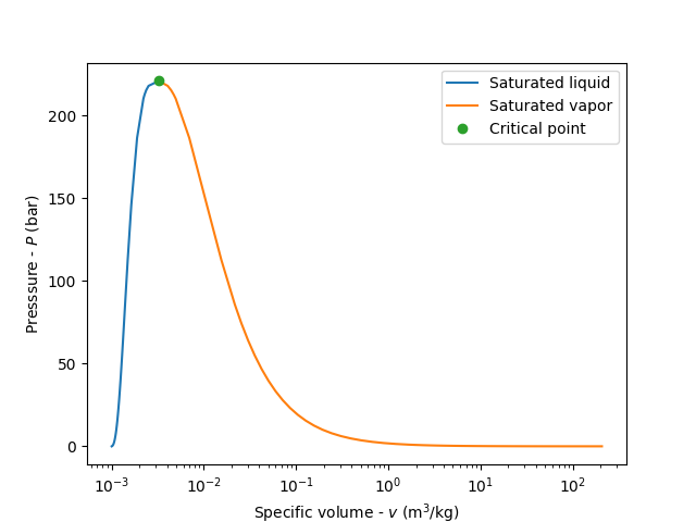
illustrate the vapor dome in a P-v diagram

plt.semilogx(df.vf.values, df.P.values, label='Saturated liquid')
plt.semilogx(df.vg.values, df.P.values, label='Saturated vapor')
plt.semilogx(df.vg.values[-1], df.P.values[-1], 'o', label='Critical point')
plt.xlabel(r'Specific volume - $v$ ($\mathrm{m^3/kg}$)')
plt.ylabel(r'Presssure - $P$ (bar)')
plt.legend();

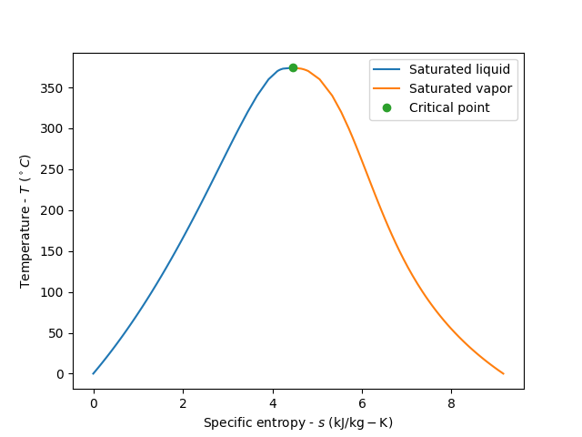
illustrate the vapor dome in a T-s diagram

plt.figure()
plt.plot(df.sf.values, df['T'].values, label='Saturated liquid')
plt.plot(df.sg.values, df['T'].values, label='Saturated vapor')
plt.plot(df.sg.values[-1], df['T'].values[-1], 'o', label='Critical point')
plt.xlabel(r'Specific entropy - $s$ ($\mathrm{kJ/kg-K}$)')
plt.ylabel(r'Temperature - $T$ (${}^\circ C$)')
plt.legend()

plt.show()