
Note
Go to the end to download the full example code.
Laminar flame speed sensitivity analysis#
In this example we simulate a freely-propagating, adiabatic, premixed methane-air flame, calculate its laminar burning velocity and perform a sensitivity analysis of its kinetics with respect to each reaction rate constant.
Requires: cantera >= 3.0.0, pandas
The figure below illustrates the setup, in a flame-fixed coordinate system. The reactants enter with density \(\rho_u\), temperature \(T_u\) and speed \(S_u\). The products exit the flame at speed \(S_b\), density \(\rho_b\) and temperature \(T_b\).

import cantera as ct
import pandas as pd
import matplotlib.pyplot as plt

plt.rcParams['figure.constrained_layout.use'] = True
Simulation parameters#
# Define the gas mixture and kinetics used to compute mixture properties
# In this case, we are using the GRI 3.0 model with methane as the fuel
mech_file = "gri30.yaml"
fuel_comp = {"CH4": 1.0}

# Inlet temperature in kelvin and inlet pressure in pascals
# In this case we are setting the inlet T and P to room temperature conditions
To = 300
Po = ct.one_atm

# Domain width in metres
width = 0.014
Simulation setup#
# Create the object representing the gas and set its state to match the inlet conditions
gas = ct.Solution(mech_file)
gas.TP = To, Po
gas.set_equivalence_ratio(1.0, fuel_comp, {"O2": 1.0, "N2": 3.76})

flame = ct.FreeFlame(gas, width=width)
flame.set_refine_criteria(ratio=3, slope=0.07, curve=0.14)
Solve the flame#
flame.solve(loglevel=1, auto=True)
************ Solving on 8 point grid with energy equation enabled ************

Attempt Newton solution of steady-state problem.
Newton steady-state solve failed.

Attempt 10 timesteps.
Final timestep info: dt= 2.136e-05  log(ss)= 5.493

Attempt Newton solution of steady-state problem.
Newton steady-state solve failed.

Attempt 10 timesteps.
Final timestep info: dt= 0.0003649  log(ss)= 4.613

Attempt Newton solution of steady-state problem.
Newton steady-state solve failed.

Attempt 10 timesteps.
Final timestep info: dt= 0.006235   log(ss)= 3.334

Attempt Newton solution of steady-state problem.
Newton steady-state solve succeeded.

Problem solved on [9] point grid(s).
Expanding domain to accommodate flame thickness. New width: 0.028 m
##############################################################################
Refining grid in flame.
    New points inserted after grid points 0 1 2 3 4 5 6 7
    to resolve C C2H C2H2 C2H3 C2H4 C2H5 C2H6 C3H7 C3H8 CH CH2 CH2(S) CH2CHO CH2CO CH2O CH2OH CH3 CH3CHO CH3O CH3OH CH4 CO CO2 H H2 H2O H2O2 HCCO HCCOH HCN HCNO HCO HNCO HO2 N N2 N2O NCO NH3 NO NO2 O O2 OH T velocity
##############################################################################

*********** Solving on 17 point grid with energy equation enabled ************

Attempt Newton solution of steady-state problem.
Newton steady-state solve failed.

Attempt 10 timesteps.
Final timestep info: dt= 2.136e-05  log(ss)= 5.75

Attempt Newton solution of steady-state problem.
Newton steady-state solve failed.

Attempt 10 timesteps.
Final timestep info: dt= 3.041e-05  log(ss)= 5.661

Attempt Newton solution of steady-state problem.
Newton steady-state solve failed.

Attempt 10 timesteps.
Final timestep info: dt= 0.0001948  log(ss)= 5.54

Attempt Newton solution of steady-state problem.
Newton steady-state solve failed.

Attempt 10 timesteps.
Final timestep info: dt= 1.951e-05  log(ss)= 6.217

Attempt Newton solution of steady-state problem.
Newton steady-state solve failed.

Attempt 10 timesteps.
Final timestep info: dt= 0.0003333  log(ss)= 5.466

Attempt Newton solution of steady-state problem.
Newton steady-state solve failed.

Attempt 10 timesteps.
Final timestep info: dt= 1.977e-05  log(ss)= 6.035

Attempt Newton solution of steady-state problem.
Newton steady-state solve succeeded.

Problem solved on [17] point grid(s).
grid refinement disabled.

******************** Solving with grid refinement enabled ********************

Attempt Newton solution of steady-state problem.
Newton steady-state solve succeeded.

Problem solved on [17] point grid(s).
##############################################################################
Refining grid in flame.
    New points inserted after grid points 3 4 5 6 7 8 9 10
    to resolve C C2H2 C2H3 C2H4 C2H5 C2H6 C3H7 C3H8 CH CH2 CH2(S) CH2CHO CH2CO CH2O CH2OH CH3 CH3CHO CH3O CH3OH CH4 CO CO2 H H2 H2O H2O2 HCCO HCCOH HCN HCNO HCO HNCO HO2 N N2 N2O NCO NH NH2 NO NO2 O O2 OH T velocity
##############################################################################

Attempt Newton solution of steady-state problem.
Newton steady-state solve failed.

Attempt 10 timesteps.
Final timestep info: dt= 0.0001709  log(ss)= 5.031

Attempt Newton solution of steady-state problem.
Newton steady-state solve succeeded.

Problem solved on [25] point grid(s).
##############################################################################
Refining grid in flame.
    New points inserted after grid points 6 7 8 9 10 11 12 13 14 15 20 21 22
    to resolve C C2H C2H2 C2H3 C2H4 C2H5 C2H6 C3H7 C3H8 CH CH2 CH2(S) CH2CHO CH2CO CH2O CH2OH CH3 CH3CHO CH3O CH3OH CH4 CO CO2 H H2 H2O H2O2 HCCO HCCOH HCN HCNO HCO HNCO HO2 N N2 N2O NCO NH NH2 NH3 NO NO2 O O2 OH T velocity
##############################################################################

Attempt Newton solution of steady-state problem.
Newton steady-state solve failed.

Attempt 10 timesteps.
Final timestep info: dt= 7.594e-05  log(ss)= 5.496

Attempt Newton solution of steady-state problem.
Newton steady-state solve succeeded.

Problem solved on [38] point grid(s).
##############################################################################
Refining grid in flame.
    New points inserted after grid points 8 9 10 11 12 13 14 15 16 17 18 19 20 21
    to resolve C C2H C2H2 C2H3 C2H4 C2H5 C2H6 C3H7 C3H8 CH CH2 CH2(S) CH2CHO CH2CO CH2O CH2OH CH3 CH3CHO CH3O CH3OH CH4 CO CO2 H H2 H2O H2O2 HCCO HCCOH HCN HCNO HCO HNCO HO2 N N2 N2O NCO NH NH2 NH3 NO NO2 O O2 OH T velocity
##############################################################################

Attempt Newton solution of steady-state problem.
Newton steady-state solve succeeded.

Problem solved on [52] point grid(s).
##############################################################################
Refining grid in flame.
    New points inserted after grid points 11 12 13 14 15 16 17 18 19 20 21 22
    to resolve C C2H C2H2 C2H3 C2H4 C2H5 C2H6 C3H7 C3H8 CH CH2 CH2(S) CH2CHO CH2CO CH2O CH2OH CH3 CH3CHO CH3O CH3OH CH4 CO CO2 H H2 H2O H2O2 HCCO HCCOH HCN HCNO HCO HNCO HO2 N N2 N2O NCO NO NO2 O O2 OH T velocity
##############################################################################

Attempt Newton solution of steady-state problem.
Newton steady-state solve succeeded.

Problem solved on [64] point grid(s).
##############################################################################
Refining grid in flame.
    New points inserted after grid points 14 15 16 17 18 19 20 21 22 23 24 25 26 27 28 29 30 31 32
    to resolve C C2H C2H2 C2H3 C2H4 C2H5 C2H6 C3H7 C3H8 CH CH2 CH2(S) CH2CHO CH2CO CH2O CH2OH CH3 CH3CHO CH3O CH3OH CH4 CO CO2 H H2 H2O H2O2 HCCO HCCOH HCN HCNO HCO HNCO HO2 N N2 NCO NO NO2 O O2 OH T velocity
##############################################################################

Attempt Newton solution of steady-state problem.
Newton steady-state solve succeeded.

Problem solved on [83] point grid(s).
##############################################################################
Refining grid in flame.
    New points inserted after grid points 19 20 21 22 23 24 25 26 27 28 29 30 31 32 33 34 35 36 37 38 39 40 41 42 43 44 45 46 47
    to resolve C C2H C2H2 C2H3 C2H4 C2H5 C2H6 C3H7 C3H8 CH CH2 CH2(S) CH2CHO CH2CO CH2O CH2OH CH3 CH3CHO CH3O CH3OH CH4 CO H H2 H2O2 HCCO HCCOH HCN HCO HNCO HO2 NO2 O OH
##############################################################################

Attempt Newton solution of steady-state problem.
Newton steady-state solve succeeded.

Problem solved on [112] point grid(s).
##############################################################################
Refining grid in flame.
    New points inserted after grid points 26 27 28 29 30 31 33 34 35 36 37 38 39 40 41 42 43 44 45 46 47 48 49 50 51 52 53 54 55 56 57 58 59 60 61 62 63 64 65 66 67 68 69 70
    to resolve C C2H2 C2H3 C2H4 C2H5 C2H6 C3H7 C3H8 CH CH2 CH2(S) CH2CHO CH2CO CH2OH CH3 CH3CHO CH3O CH3OH H2O2 HCCO HCCOH HCO HO2
##############################################################################

Attempt Newton solution of steady-state problem.
Newton steady-state solve succeeded.

Problem solved on [156] point grid(s).
no new points needed in flame
print(f"\nmixture-averaged flame speed = {flame.velocity[0]:7f} m/s\n")
mixture-averaged flame speed = 0.381286 m/s
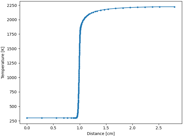
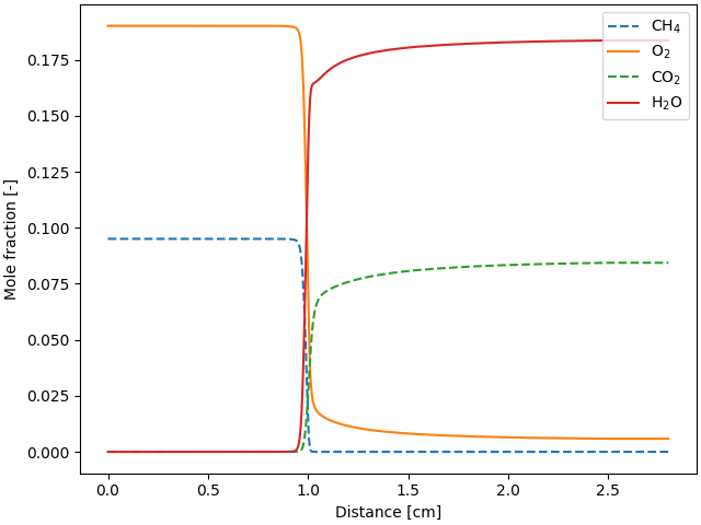
Plot temperature and major species profiles#
Check and see if all has gone well.
# Extract the spatial profiles as a SolutionArray to simplify plotting specific species
profile = flame.to_array()

fig, ax = plt.subplots()

ax.plot(profile.grid * 100, profile.T, ".-")
ax.set_xlabel("Distance [cm]")
ax.set_ylabel("Temperature [K]")
fig, ax = plt.subplots()

ax.plot(profile.grid * 100, profile("CH4").X, "--", label="CH$_4$")
ax.plot(profile.grid * 100, profile("O2").X, label="O$_2$")
ax.plot(profile.grid * 100, profile("CO2").X, "--", label="CO$_2$")
ax.plot(profile.grid * 100, profile("H2O").X, label="H$_2$O")

ax.legend(loc="best")
ax.set_xlabel("Distance [cm]")
ax.set_ylabel("Mole fraction [-]")
plt.show()
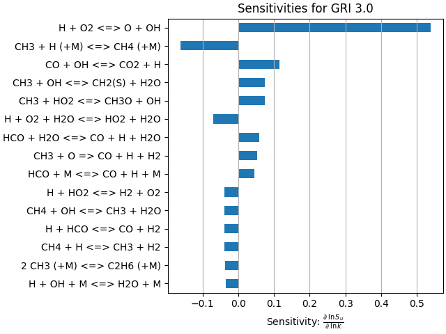
Sensitivity Analysis#
See which reactions affect the flame speed the most. The sensitivities can be efficiently computed using the adjoint method. In the general case, we consider a system \(f(x, p) = 0\) where \(x\) is the system’s state vector and \(p\) is a vector of parameters. To compute the sensitivities of a scalar function \(g(x, p)\) to the parameters, we solve the system:
for the Lagrange multiplier vector \(\lambda\). The sensitivities are then computed as
In the case of flame speed sensitivity to the reaction rate coefficients, \(g = S_u\) and \(\partial g/\partial p = 0\). Since \(\partial f/\partial x\) is already computed as part of the normal solution process, computing the sensitivities for \(N\) reactions only requires \(N\) additional evaluations of the residual function to obtain \(\partial f/\partial p\), plus the solution of the linear system for \(\lambda\).
Calculation of flame speed sensitivities with respect to rate coefficients is
implemented by the method FreeFlame.get_flame_speed_reaction_sensitivities. For
other sensitivities, the method Sim1D.solve_adjoint can be used.
# Create a DataFrame to store sensitivity-analysis data
sens = pd.DataFrame(index=gas.reaction_equations(), columns=["sensitivity"])

# Use the adjoint method to calculate sensitivities
sens.sensitivity = flame.get_flame_speed_reaction_sensitivities()

# Show the first 10 sensitivities
sens.head(10)
# Sort the sensitivities in order of descending magnitude
sens = sens.iloc[(-sens['sensitivity'].abs()).argsort()]

fig, ax = plt.subplots()

# Reaction mechanisms can contains thousands of elementary steps. Limit the plot
# to the top 15
sens.head(15).plot.barh(ax=ax, legend=None)

ax.invert_yaxis()  # put the largest sensitivity on top
ax.set_title("Sensitivities for GRI 3.0")
ax.set_xlabel(r"Sensitivity: $\frac{\partial\:\ln S_u}{\partial\:\ln k}$")
ax.grid(axis='x')
plt.show()
Total running time of the script: (0 minutes 9.081 seconds)