Blowers-Masel reaction rates

A simple example to demonstrate the difference between Blowers-Masel reaction and elementary reaction.

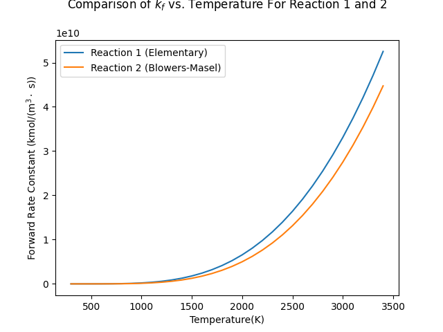
First we show that the forward rate constants of the first 2 different reactions are different because of the different rate expression, then we print the forward rate constants for reaction 2 and reaction 3 to show that even two reactions that have the same Blowers-Masel parameters can have different forward rate constants.

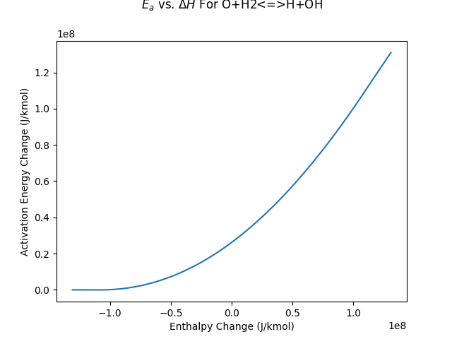
The first plot generated shows how the rate constant changes with respect to temperature for elementary and Blower-Masel reactions. The second plot shows the activation energy change of a Blowers-Masel reaction with respect to the delta enthalpy of the reaction.

Requires: cantera >= 2.6.0, matplotlib >= 2.0

Tags: Python kinetics sensitivity analysis

import cantera as ct
import numpy as np
import matplotlib.pyplot as plt

Create an elementary reaction:

r1 = ct.Reaction(equation="O + H2 <=> H + OH",
                 rate=ct.ArrheniusRate(3.87e1, 2.7, 6260*1000*4.184))

Create a Blowers-Masel reaction:

r2 = ct.Reaction(equation="O + H2 <=> H + OH",
                 rate=ct.BlowersMaselRate(3.87e1, 2.7, 6260*1000*4.184, 1e9))

Create a Blowers-Masel reaction with same parameters as r2, but for different reactants and products

r3 = ct.Reaction(equation="H + CH4 <=> CH3 + H2",
                 rate=ct.BlowersMaselRate(3.87e1, 2.7, 6260*1000*4.184, 1e9))

Evaluate these reaction rates as part of a gas mixture

gas = ct.Solution(thermo='ideal-gas', kinetics='gas',
                  species=ct.Solution('gri30.yaml').species(), reactions=[r1, r2, r3])

gas.TP = 300, ct.one_atm

r1_rc = gas.forward_rate_constants[0]
r2_rc = gas.forward_rate_constants[1]
r3_rc = gas.forward_rate_constants[2]

The first two reactions have the same reaction equations with Arrhenius and Blowers-Masel rate parameters, respectively. The Blowers-Masel parameters are the same as the Arrhenius parameters with an additional value, bond energy. The forward rate constants for these two reactions are different because of the difference in the rate expression:

print(f"{r1_rc=:.3f} kmol/m³/s")
print(f"{r2_rc=:.3f} kmol/m³/s")

r1_rc=5195.447 kmol/m³/s
r2_rc=946.051 kmol/m³/s

The rate parameters of second and the third reactions are same, but their reactants and products are different. Since the enthalpy of reaction is used in the Blowers-Masel rate expression, the rate constants are different:

print(f"{r2_rc=:.3f} kmol/m³/s")
print(f"{r3_rc=:.3f} kmol/m³/s")

r2_rc=946.051 kmol/m³/s
r3_rc=2533.800 kmol/m³/s

Effect of temperature on reaction rates

Compare the reaction forward rate constant change of Blowers-Masel reaction and elementary reaction with respect to the temperature.

r1_kf = []
r2_kf = []
T_range = np.arange(300, 3500, 100)
for temp in T_range:
    gas.TP = temp, ct.one_atm
    r1_kf.append(gas.forward_rate_constants[0])
    r2_kf.append(gas.forward_rate_constants[1])

fig, ax = plt.subplots()
ax.plot(T_range, r1_kf, label='Reaction 1 (Elementary)')
ax.plot(T_range, r2_kf, label='Reaction 2 (Blowers-Masel)')
ax.set(xlabel="Temperature(K)", ylabel=r"Forward Rate Constant (kmol/(m$^3\cdot$ s))")
ax.set_title("Comparison of $k_f$ vs. Temperature For Reaction 1 and 2")
ax.legend()
plt.savefig("kf_to_T.png")
plt.show()

Plot the activation energy change of reaction 2 with respect to the enthalpy change

# This is the function to change the enthalpy of a species
# so that the enthalpy change of reactions involving this species can be changed
def change_species_enthalpy(gas, species_name, dH):
    """
    Find the species by name and change it's enthalpy by dH (in J/kmol)
    """
    index = gas.species_index(species_name)

    species = gas.species(index)
    # dx is in fact (delta H / R). Note that R in cantera is 8314.462 J/kmol/K
    dx = dH / ct.gas_constant
    perturbed_coeffs = species.thermo.coeffs.copy()
    perturbed_coeffs[6] += dx
    perturbed_coeffs[13] += dx

    species.thermo = ct.NasaPoly2(species.thermo.min_temp, species.thermo.max_temp,
                                  species.thermo.reference_pressure, perturbed_coeffs)

    gas.modify_species(index, species)
    return gas.delta_enthalpy[1]

E0 = gas.reaction(1).rate.activation_energy
upper_limit_enthalpy = 5 * E0
lower_limit_enthalpy = -5 * E0

Ea_list = []
deltaH_list = np.linspace(lower_limit_enthalpy, upper_limit_enthalpy, 100)
for deltaH in deltaH_list:
    delta_enthalpy = change_species_enthalpy(gas, "H", deltaH - gas.delta_enthalpy[1])
    gas.reaction(1).rate.delta_enthalpy = delta_enthalpy
    Ea_list.append(gas.reaction(1).rate.activation_energy)

fig, ax = plt.subplots()
ax.plot(deltaH_list, Ea_list)
ax.set(xlabel="Enthalpy Change (J/kmol)", ylabel="Activation Energy Change (J/kmol)")
ax.set_title(r"$E_a$ vs. $\Delta H$ For $\mathrm{ O+H_2 \rightleftharpoons H+OH }$")
plt.savefig("Ea_to_H.png")
plt.show()