Integrating constant pressure ignition using SciPy

Solve a constant pressure ignition problem in Python using an external integrator.

This demonstrates an approach for solving problems where Cantera is used to evaluate thermodynamic properties and kinetic rates while an external ODE solver is used to integrate the resulting equations. In this case, the SciPy wrapper for VODE is used, which uses the same variable-order BDF methods as the Sundials CVODES solver used by Cantera. For most cases that are only modest variations on the standard reactor types, the extensible reactor framework provides an approach that builds on Cantera’s existing reactor network capabilities.

Requires: cantera >= 2.5.0, scipy >= 0.19, matplotlib >= 2.0

Tags: Python combustion reactor network ignition delay user-defined model plotting

import cantera as ct
import numpy as np
import scipy.integrate


class ReactorOde:
    def __init__(self, gas):
        # Parameters of the ODE system and auxiliary data are stored in the
        # ReactorOde object.
        self.gas = gas
        self.P = gas.P

    def __call__(self, t, y):
        """the ODE function, y' = f(t,y) """

        # State vector is [T, Y_1, Y_2, ... Y_K]
        self.gas.set_unnormalized_mass_fractions(y[1:])
        self.gas.TP = y[0], self.P
        rho = self.gas.density

        wdot = self.gas.net_production_rates
        dTdt = - (np.dot(self.gas.partial_molar_enthalpies, wdot) /
                  (rho * self.gas.cp))
        dYdt = wdot * self.gas.molecular_weights / rho

        return np.hstack((dTdt, dYdt))


gas = ct.Solution('h2o2.yaml')

# Initial condition
P = ct.one_atm
gas.TPX = 1001, P, 'H2:2,O2:1,N2:4'
y0 = np.hstack((gas.T, gas.Y))

# Set up objects representing the ODE and the solver
ode = ReactorOde(gas)
solver = scipy.integrate.ode(ode)
solver.set_integrator('vode', method='bdf', with_jacobian=True)
solver.set_initial_value(y0, 0.0)

# Integrate the equations, keeping T(t) and Y(k,t)
t_end = 1e-3
states = ct.SolutionArray(gas, 1, extra={'t': [0.0]})
dt = 1e-5
while solver.successful() and solver.t < t_end:
    solver.integrate(solver.t + dt)
    gas.TPY = solver.y[0], P, solver.y[1:]
    states.append(gas.state, t=solver.t)

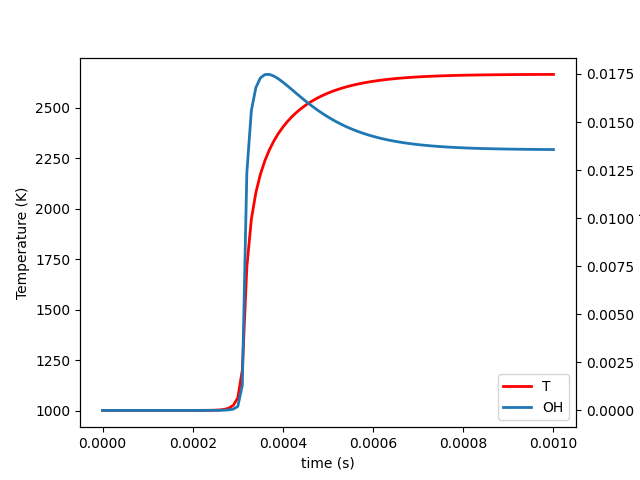
# Plot the results
try:
    import matplotlib.pyplot as plt
    L1 = plt.plot(states.t, states.T, color='r', label='T', lw=2)
    plt.xlabel('time (s)')
    plt.ylabel('Temperature (K)')
    plt.twinx()
    L2 = plt.plot(states.t, states('OH').Y, label='OH', lw=2)
    plt.ylabel('Mass Fraction')
    plt.legend(L1+L2, [line.get_label() for line in L1+L2], loc='lower right')
    plt.show()
except ImportError:
    print('Matplotlib not found. Unable to plot results.')