Acceleration of reactor integration using a sparse preconditioned solver

Ideal gas, constant-pressure, adiabatic kinetics simulation that compares preconditioned and non-preconditioned integration of nDodecane.

Requires: cantera >= 3.0.0, matplotlib >= 2.0

Tags: Python combustion reactor network preconditioner

Preconditioned Integration Time: 0.119947
steps 1040
rhs_evals 1191
nonlinear_iters 1188
nonlinear_conv_fails 4
err_test_fails 26
last_order 3
stab_order_reductions 0
jac_evals 0
lin_solve_setups 98
lin_rhs_evals 3242
lin_iters 3242
lin_conv_fails 75
prec_evals 21
prec_solves 4329
jt_vec_setup_evals 0
jt_vec_prod_evals 3242


Non-preconditioned Integration Time: 0.264189
steps 3043
rhs_evals 5243
nonlinear_iters 5240
nonlinear_conv_fails 34
err_test_fails 214
last_order 3
stab_order_reductions 0
jac_evals 65
lin_solve_setups 451
lin_rhs_evals 6565
lin_iters 0
lin_conv_fails 0
prec_evals 0
prec_solves 0
jt_vec_setup_evals 0
jt_vec_prod_evals 0

import cantera as ct
import numpy as np
import matplotlib.pyplot as plt
from timeit import default_timer

def integrate_reactor(n_reactors=1, preconditioner=True):
    """
        Compare the integrations of a preconditioned reactor network and a
        non-preconditioned reactor network. Increase the number of reactors in the
        network with the keyword argument `n_reactors` to see greater differences in
        performance.
    """
    # Use a reduced n-dodecane mechanism with PAH formation pathways
    gas = ct.Solution('nDodecane_Reitz.yaml', 'nDodecane_IG')
    # Create multiple reactors and set initial contents
    gas.TP = 1000, ct.one_atm
    gas.set_equivalence_ratio(1, 'c12h26', 'n2:3.76, o2:1.0')
    reactors = [ct.IdealGasConstPressureMoleReactor(gas) for n in range(n_reactors)]
    # set volume for reactors
    for r in reactors:
        r.volume = 0.1
    # Create reactor network
    sim = ct.ReactorNet(reactors)
    # Add preconditioner
    if preconditioner:
        sim.derivative_settings = {"skip-third-bodies":True, "skip-falloff":True}
        sim.preconditioner = ct.AdaptivePreconditioner()
    sim.initialize()
    # Advance to steady state
    integ_time = default_timer()
    # solution array for state data
    states = ct.SolutionArray(reactors[0].thermo, extra=['time'])
    # advance to steady state manually
    while (sim.time < 0.1):
        states.append(reactors[0].thermo.state, time=sim.time)
        sim.step()
    integ_time = default_timer() - integ_time
    # Return time to integrate
    if preconditioner:
        print(f"Preconditioned Integration Time: {integ_time:f}")
    else:
        print(f"Non-preconditioned Integration Time: {integ_time:f}")
    # Get and output solver stats
    for key, value in sim.solver_stats.items():
        print(key, value)
    print("\n")
    # return some variables for plotting
    return states.time, states.T, states('CO2').Y, states('C12H26').Y

if __name__ == "__main__":
    # integrate both to steady state
    timep, Tp, CO2p, C12H26p = integrate_reactor(preconditioner=True)
    timenp, Tnp, CO2np, C12H26np  = integrate_reactor(preconditioner=False)
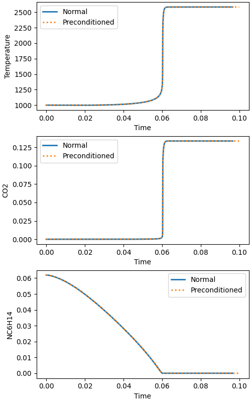
    # plot selected state variables
    fig, axs = plt.subplots(1, 3)
    fig.tight_layout()
    ax1, ax2, ax3 = axs
    # temperature plot
    ax1.set_xlabel("Time")
    ax1.set_ylabel("Temperature")
    ax1.plot(timenp, Tnp, linewidth=2)
    ax1.plot(timep, Tp, linewidth=2, linestyle=":")
    ax1.legend(["Normal", "Preconditioned"])
    # CO2 plot
    ax2.set_xlabel("Time")
    ax2.set_ylabel("CO2")
    ax2.plot(timenp, CO2np, linewidth=2)
    ax2.plot(timep, CO2p, linewidth=2, linestyle=":")
    ax2.legend(["Normal", "Preconditioned"])
    # C12H26 plot
    ax3.set_xlabel("Time")
    ax3.set_ylabel("C12H26")
    ax3.plot(timenp, C12H26np, linewidth=2)
    ax3.plot(timep, C12H26p, linewidth=2, linestyle=":")
    ax3.legend(["Normal", "Preconditioned"])
    plt.show()