Ignition delay time using the Redlich-Kwong real gas model

In this example we illustrate how to setup and use a constant volume, adiabatic reactor to simulate reflected shock tube experiments. This reactor is then used to compute the ignition delay of a gas at a specified initial temperature and pressure.

The example is written in a general way, that is, no particular equation of state (EoS) is presumed and ideal and real gas EoS can be used equally easily. The example here demonstrates the calculations carried out by G. Kogekar et al. [1].

Requires: cantera >= 2.5.0, matplotlib >= 2.0

Tags: Python combustion reactor network non-ideal fluid ignition delay plotting

Methods

Reflected Shock Reactor

The reflected shock tube reactor is modeled as a closed, constant-volume, adiabatic reactor. The heat transfer and the work rates are therefore both zero. With no mass inlets or exits, the 1st law energy balance reduces to:

\[\frac{dU}{dt} = \dot{Q} - \dot{W} = 0\]

Because of the constant-mass and constant-volume assumptions, the density is also therefore constant:

\[\frac{d\rho}{dt} = 0\]

Along with the evolving gas composition, the thermodynamic state of the gas is defined by the initial total internal energy \(U = m u = m \sum_k Y_k u_k\), where \(u_k\) and \(Y_k\) are the specific internal energy (J/kg) and mass fraction of species \(k\), respectively.

The species mass fractions evolve according to the net chemical production rates due to homogeneous gas-phase reactions:

\[\frac{dY_k}{dt} = \frac{W_k}{\rho}\dot{\omega}_k,\]

where \(W_k\) is the molecular weight of species \(k\) (kg/kmol³), \(\rho\) is the (constant) gas-phase density (kg/m³), and \(\dot{\omega}_k\) is the net production rate of species \(k\) (kmol/m³/s).

Redlich-Kwong Parameters

Redlich-Kwong constants for each species are calculated according to their critical temperature \(T_c\) and pressure \(P_c\):

\[a = 0.4275 \frac{R^2 T_c^{2.5}}{P_c}\]

and

\[b = 0.08664 \frac{R T_c}{P_c}\]

where \(R\) is the universal gas constant.

For stable species, the critical properties are readily available. For radicals and other short-lived intermediates, the Joback method [3] is used to estimate critical properties.

# Dependencies: numpy, and matplotlib
import numpy as np
import matplotlib.pyplot as plt

import time

import cantera as ct
print('Running Cantera version: ' + ct.__version__)

Running Cantera version: 3.1.0a2

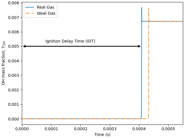
Define the ignition delay time (IDT). This function computes the ignition delay from the occurrence of the peak concentration for the specified species.

def ignition_delay(states, species):
    i_ign = states(species).Y.argmax()
    return states.t[i_ign]

Define initial conditions and reaction mechanism

In this example we will choose a stoichiometric mixture of n-dodecane and air as the gas. For a representative kinetic model, we use the one from Wang et al [2].

# Define the reactor temperature and pressure:
reactor_temperature = 1000  # Kelvin
reactor_pressure = 40.0*101325.0  # Pascals

# Load the real gas mechanism:
real_gas = ct.Solution('nDodecane_Reitz.yaml', 'nDodecane_RK')

# Create the ideal gas object:
ideal_gas = ct.Solution('nDodecane_Reitz.yaml', 'nDodecane_IG')

Real gas IDT calculation

# Set the state of the gas object:
real_gas.TP = reactor_temperature, reactor_pressure

# Define the fuel, oxidizer and set the stoichiometry:
real_gas.set_equivalence_ratio(phi=1.0, fuel='c12h26',
                               oxidizer={'o2': 1.0, 'n2': 3.76})

# Create a reactor object and add it to a reactor network
# In this example, this will be the only reactor in the network
r = ct.Reactor(contents=real_gas)
reactor_network = ct.ReactorNet([r])
time_history_RG = ct.SolutionArray(real_gas, extra=['t'])

# This is a starting estimate. If you do not get an ignition within this time,
# increase it
estimated_ignition_delay_time = 0.005

t = 0
t0 = time.time()
counter = 1
while t < estimated_ignition_delay_time:
    t = reactor_network.step()
    if counter % 20 == 0:
        # We will save only every 20th value. Otherwise, this takes too long
        # Note that the species concentrations are mass fractions
        time_history_RG.append(r.thermo.state, t=t)
    counter += 1

# We will use the 'oh' species to compute the ignition delay
tau_RG = ignition_delay(time_history_RG, 'oh')

t1 = time.time()
print("Computed Real Gas Ignition Delay: {:.3e} seconds. "
      "Took {:3.2f} s to compute".format(tau_RG, t1-t0))

Computed Real Gas Ignition Delay: 4.093e-04 seconds. Took 5.14 s to compute

Ideal gas IDT calculation

# Set the state of the gas object:
ideal_gas.TP = reactor_temperature, reactor_pressure

# Define the fuel, oxidizer and set the stoichiometry:
ideal_gas.set_equivalence_ratio(phi=1.0, fuel='c12h26',
                                oxidizer={'o2': 1.0, 'n2': 3.76})

r = ct.Reactor(contents=ideal_gas)
reactor_network = ct.ReactorNet([r])
time_history_IG = ct.SolutionArray(ideal_gas, extra=['t'])

t0 = time.time()
t = 0
counter = 1
while t < estimated_ignition_delay_time:
    t = reactor_network.step()
    if counter % 20 == 0:
        # We will save only every 20th value. Otherwise, this takes too long
        # Note that the species concentrations are mass fractions
        time_history_IG.append(r.thermo.state, t=t)
    counter += 1

# We will use the 'oh' species to compute the ignition delay
tau_IG = ignition_delay(time_history_IG, 'oh')
t1 = time.time()

print("Computed Ideal Gas Ignition Delay: {:.3e} seconds. "
      "Took {:3.2f} s to compute".format(tau_IG, t1-t0))
print('Ideal gas error: {:2.2f} %'.format(100*(tau_IG-tau_RG)/tau_RG))

Computed Ideal Gas Ignition Delay: 4.333e-04 seconds. Took 0.35 s to compute
Ideal gas error: 5.86 %

Plot the results

plt.rcParams['figure.constrained_layout.use'] = True

# Figure illustrating the definition of ignition delay time (IDT).
plt.figure()
plt.plot(time_history_RG.t, time_history_RG('oh').Y)
plt.plot(time_history_IG.t, time_history_IG('oh').Y, '-.')
plt.xlabel('Time (s)')
plt.ylabel(r'OH mass fraction, $\mathdefault{Y_{OH}}$')

# Figure formatting:
plt.xlim([0, 0.00055])
ax = plt.gca()
ax.annotate("", xy=(tau_RG, 0.005), xytext=(0, 0.005),
            arrowprops=dict(arrowstyle="<|-|>", color='k', linewidth=2.0))
plt.annotate('Ignition Delay Time (IDT)', xy=(0, 0), xytext=(0.00008, 0.00525))

plt.legend(['Real Gas', 'Ideal Gas'])

# If you want to save the plot, uncomment this line (and edit as you see fit):
# plt.savefig('IDT_nDodecane_1000K_40atm.pdf', dpi=350, format='pdf')

Demonstration of NTC behavior

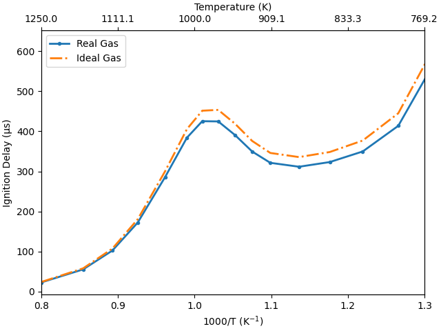
A common benchmark for a reaction mechanism is its ability to reproduce the negative temperature coefficient (NTC) behavior. Intuitively, as the temperature of an explosive mixture increases, it should ignite faster. But, under certain conditions, we observe the opposite. This is referred to as NTC behavior. Reproducing experimentally observed NTC behavior is thus an important test for any mechanism. We will do this now by computing and visualizing the ignition delay for a wide range of temperatures

# Make a list of all the temperatures at which we would like to run simulations:
T = np.array([1250, 1170, 1120, 1080, 1040, 1010, 990, 970, 950, 930, 910, 880, 850,
              820, 790, 760])

# If we desire, we can define different IDT starting guesses for each temperature:
estimated_ignition_delay_times = np.ones(len(T))
# But we won't, at least in this example :)
estimated_ignition_delay_times[:] = 0.005

# Now, we simply run the code above for each temperature.
# Real Gas
ignition_delays_RG = np.zeros(len(T))
for i, temperature in enumerate(T):
    # Setup the gas and reactor
    reactor_temperature = temperature
    real_gas.TP = reactor_temperature, reactor_pressure
    real_gas.set_equivalence_ratio(phi=1.0, fuel='c12h26',
                                   oxidizer={'o2': 1.0, 'n2': 3.76})
    r = ct.Reactor(contents=real_gas)
    reactor_network = ct.ReactorNet([r])

    # create an array of solution states
    time_history = ct.SolutionArray(real_gas, extra=['t'])

    t0 = time.time()
    t = 0
    counter = 1
    while t < estimated_ignition_delay_times[i]:
        t = reactor_network.step()
        if counter % 20 == 0:
            time_history.append(r.thermo.state, t=t)
        counter += 1

    tau = ignition_delay(time_history, 'oh')
    t1 = time.time()

    print("Computed Real Gas Ignition Delay: {:.3e} seconds for T={:.1f} K. "
          "Took {:3.2f} s to compute".format(tau, temperature, t1-t0))

    ignition_delays_RG[i] = tau


# Repeat for Ideal Gas
ignition_delays_IG = np.zeros(len(T))
for i, temperature in enumerate(T):
    # Setup the gas and reactor
    reactor_temperature = temperature
    ideal_gas.TP = reactor_temperature, reactor_pressure
    ideal_gas.set_equivalence_ratio(phi=1.0, fuel='c12h26',
                                    oxidizer={'o2': 1.0, 'n2': 3.76})
    r = ct.Reactor(contents=ideal_gas)
    reactor_network = ct.ReactorNet([r])

    # create an array of solution states
    time_history = ct.SolutionArray(ideal_gas, extra=['t'])

    t0 = time.time()

    t = 0
    counter = 1
    while t < estimated_ignition_delay_times[i]:
        t = reactor_network.step()
        if counter % 20 == 0:
            time_history.append(r.thermo.state, t=t)
        counter += 1

    tau = ignition_delay(time_history, 'oh')
    t1 = time.time()

    print("Computed Ideal Gas Ignition Delay: {:.3e} seconds for T={:.1f} K. "
          "Took {:3.2f} s to compute".format(tau, temperature, t1-t0))

    ignition_delays_IG[i] = tau

Computed Real Gas Ignition Delay: 2.274e-05 seconds for T=1250.0 K. Took 4.09 s to compute
Computed Real Gas Ignition Delay: 5.532e-05 seconds for T=1170.0 K. Took 4.35 s to compute
Computed Real Gas Ignition Delay: 1.024e-04 seconds for T=1120.0 K. Took 4.54 s to compute
Computed Real Gas Ignition Delay: 1.723e-04 seconds for T=1080.0 K. Took 4.99 s to compute
Computed Real Gas Ignition Delay: 2.857e-04 seconds for T=1040.0 K. Took 5.03 s to compute
Computed Real Gas Ignition Delay: 3.842e-04 seconds for T=1010.0 K. Took 4.98 s to compute
Computed Real Gas Ignition Delay: 4.254e-04 seconds for T=990.0 K. Took 5.12 s to compute
Computed Real Gas Ignition Delay: 4.248e-04 seconds for T=970.0 K. Took 5.24 s to compute
Computed Real Gas Ignition Delay: 3.911e-04 seconds for T=950.0 K. Took 5.61 s to compute
Computed Real Gas Ignition Delay: 3.496e-04 seconds for T=930.0 K. Took 5.51 s to compute
Computed Real Gas Ignition Delay: 3.214e-04 seconds for T=910.0 K. Took 5.78 s to compute
Computed Real Gas Ignition Delay: 3.116e-04 seconds for T=880.0 K. Took 5.65 s to compute
Computed Real Gas Ignition Delay: 3.233e-04 seconds for T=850.0 K. Took 6.13 s to compute
Computed Real Gas Ignition Delay: 3.498e-04 seconds for T=820.0 K. Took 6.09 s to compute
Computed Real Gas Ignition Delay: 4.138e-04 seconds for T=790.0 K. Took 6.32 s to compute
Computed Real Gas Ignition Delay: 5.819e-04 seconds for T=760.0 K. Took 6.34 s to compute
Computed Ideal Gas Ignition Delay: 2.380e-05 seconds for T=1250.0 K. Took 0.29 s to compute
Computed Ideal Gas Ignition Delay: 5.794e-05 seconds for T=1170.0 K. Took 0.33 s to compute
Computed Ideal Gas Ignition Delay: 1.073e-04 seconds for T=1120.0 K. Took 0.33 s to compute
Computed Ideal Gas Ignition Delay: 1.806e-04 seconds for T=1080.0 K. Took 0.34 s to compute
Computed Ideal Gas Ignition Delay: 3.001e-04 seconds for T=1040.0 K. Took 0.34 s to compute
Computed Ideal Gas Ignition Delay: 4.057e-04 seconds for T=1010.0 K. Took 0.34 s to compute
Computed Ideal Gas Ignition Delay: 4.516e-04 seconds for T=990.0 K. Took 0.37 s to compute
Computed Ideal Gas Ignition Delay: 4.536e-04 seconds for T=970.0 K. Took 0.37 s to compute
Computed Ideal Gas Ignition Delay: 4.194e-04 seconds for T=950.0 K. Took 0.39 s to compute
Computed Ideal Gas Ignition Delay: 3.760e-04 seconds for T=930.0 K. Took 0.38 s to compute
Computed Ideal Gas Ignition Delay: 3.461e-04 seconds for T=910.0 K. Took 0.38 s to compute
Computed Ideal Gas Ignition Delay: 3.357e-04 seconds for T=880.0 K. Took 0.41 s to compute
Computed Ideal Gas Ignition Delay: 3.484e-04 seconds for T=850.0 K. Took 0.41 s to compute
Computed Ideal Gas Ignition Delay: 3.772e-04 seconds for T=820.0 K. Took 0.42 s to compute
Computed Ideal Gas Ignition Delay: 4.452e-04 seconds for T=790.0 K. Took 0.44 s to compute
Computed Ideal Gas Ignition Delay: 6.215e-04 seconds for T=760.0 K. Took 0.46 s to compute

# Figure: ignition delay (tau) vs. the inverse of temperature (1000/T).
fig, ax = plt.subplots()
ax.plot(1000/T, 1e6*ignition_delays_RG, '.-', linewidth=2.0)
ax.plot(1000/T, 1e6*ignition_delays_IG, '-.', linewidth=2.0)
ax.set_ylabel(r'Ignition Delay (μs)')
ax.set_xlabel(r'1000/T (K$^{-1}$)')

ax.set_xlim([0.8, 1.3])

# Add a second axis on top to plot the temperature for better readability
ax2 = ax.twiny()
ticks = ax.get_xticks()
ax2.set_xticks(ticks)
ax2.set_xticklabels((1000/ticks).round(1))
ax2.set_xlim(ax.get_xlim())
ax2.set_xlabel('Temperature (K)')

ax.legend(['Real Gas', 'Ideal Gas'], loc='upper left')

# If you want to save the plot, uncomment this line (and edit as you see fit):
# plt.savefig('NTC_nDodecane_40atm.pdf', dpi=350, format='pdf')

# Show the plots.
plt.show()

References

[1]

G. Kogekar, C. Karakaya, G. J. Liskovich, M. A. Oehlschlaeger, S. C. DeCaluwe, R. J. Kee (2018). “Impact of non-ideal behavior on ignition delay and chemical kinetics in high-pressure shock tube reactors,” Combust. Flame. 189 1-11, https://doi.org/10.1016/j.combustflame.2017.10.014

[2]

H. Wang, Y. Ra, M. Jia, R. Reitz (2014). “Development of a reduced n-dodecane-PAH mechanism and its application for n-dodecane soot predictions”, Fuel 136, 25–36. https://doi.org/10.1016/j.fuel.2014.07.028.

[3]

K. G. Joback and R. C. Reid (1987). “Estimation of pure-component properties from group-contributions,” Chem. Eng. Comm. 57, 233-243, https://doi.org/10.1080/00986448708960487.