Continuously stirred tank reactor with periodic behavior

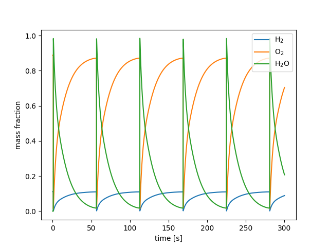
This example illustrates a continuously stirred tank reactor (CSTR) with steady inputs but periodic interior state.

A stoichiometric hydrogen/oxygen mixture is introduced and reacts to produce water. But since water has a large efficiency as a third body in the chain termination reaction

\[\mathrm{ H + O_2 + M \rightleftharpoons HO_2 + M }\]

as soon as a significant amount of water is produced the reaction stops. After enough time has passed that the water is exhausted from the reactor, the mixture explodes again and the process repeats. This explanation can be verified by decreasing the rate for reaction 7 in file h2o2.yaml and re-running the example.

Acknowledgments: The idea for this example and an estimate of the conditions needed to see the oscillations came from Bob Kee, Colorado School of Mines

Requires: cantera >= 2.5.0, matplotlib >= 2.0

Tags: Python combustion reactor network well-stirred reactor plotting

import cantera as ct
import matplotlib.pyplot as plt

Create the gas mixture and set initial conditions

gas = ct.Solution('h2o2.yaml')

# pressure = 60 Torr, T = 770 K
p = 60.0*133.3
t = 770.0

gas.TPX = t, p, 'H2:2, O2:1'

Create an upstream reservoir that will supply the reactor. The temperature, pressure, and composition of the upstream reservoir are set to those of the gas object at the time the reservoir is created.

upstream = ct.Reservoir(gas)

Now create the reactor object with the same initial state.

Set its volume to 10 cm³. In this problem, the reactor volume is fixed, so the initial volume is the volume at all later times.

cstr = ct.IdealGasReactor(gas)
cstr.volume = 10.0*1.0e-6

We need to have heat loss to see the oscillations. Create a reservoir to represent the environment, and initialize its temperature to the reactor temperature.

env = ct.Reservoir(gas)

Create a heat-conducting wall between the reactor and the environment. Set its area, and its overall heat transfer coefficient. Larger U causes the reactor to be closer to isothermal. If U is too small, the gas ignites, and the temperature spikes and stays high.

w = ct.Wall(cstr, env, A=1.0, U=0.02)

Connect the upstream reservoir to the reactor with a mass flow controller (constant mdot). Set the mass flow rate to 1.25 sccm.

sccm = 1.25
vdot = sccm * 1.0e-6 / 60.0 * ((ct.one_atm / gas.P) * (gas.T / 273.15))  # m^3/s
mdot = gas.density * vdot  # kg/s
mfc = ct.MassFlowController(upstream, cstr, mdot=mdot)

Now create a downstream reservoir to exhaust into and connect the reactor to this reservoir with a valve. Set the coefficient sufficiently large to keep the reactor pressure close to the downstream pressure of 60 Torr.

downstream = ct.Reservoir(gas)
v = ct.Valve(cstr, downstream, K=1.0e-9)

Create the network and integrate in time:

network = ct.ReactorNet([cstr])
t = 0.0
dt = 0.1

states = ct.SolutionArray(gas, extra=['t'])
while t < 300.0:
    t += dt
    network.advance(t)
    states.append(cstr.thermo.state, t=t)

aliases = {'H2': 'H$_2$', 'O2': 'O$_2$', 'H2O': 'H$_2$O'}
for name, alias in aliases.items():
    gas.add_species_alias(name, alias)

fig, ax = plt.subplots()
for spc in aliases.values():
    ax.plot(states.t, states(spc).Y, label=spc)
plt.legend(loc='upper right')
plt.xlabel('time [s]')
plt.ylabel('mass fraction')
plt.show()