

Note
Go to the end to download the full example code.
Preconditioned integration of a coupled reactor network#
This example demonstrates the effect of including cross-reactor Jacobian terms from walls and flow devices in the sparse preconditioner matrix.
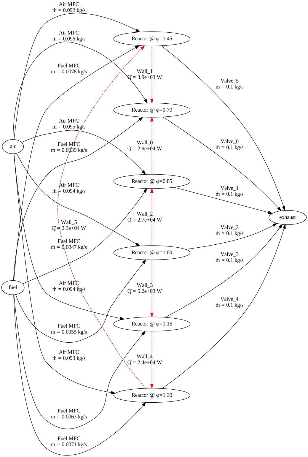
The network represents the sectors of a simplified annular combustor with non-uniform fuel/air mixing. A single methane supply and a single air supply feed each sector through a pair of mass flow controllers, with the relative flow split set to give each sector a distinct equivalence ratio — as would happen if the fuel injectors around the combustor were running at slightly different operating points. All sectors vent to a shared exhaust and adjacent sectors are separated by thin metal liner walls with high heat transfer. The strong wall coupling drives all sectors toward a nearly uniform temperature while the equivalence-ratio variation keeps the species distributions distinct.
Four integration strategies are compared:
Preconditioned, with wall and flow-device Jacobian terms included (default)
Preconditioned, with wall terms excluded (
skip-wallsoption)Preconditioned, with flow-device terms excluded (
skip-flow-devicesoption)Direct integration without preconditioning
Both the wall coupling and the flow-device coupling introduce significant cross-reactor entries in the Jacobian. Omitting either set of terms substantially increases the number of Krylov iterations and integrator step rejections; in this network, dropping the wall terms is enough to make the preconditioned solve slower than direct integration with no preconditioning at all.
Requires: cantera >= 4.0.0, matplotlib >= 2.0
import cantera as ct
import matplotlib.pyplot as plt
from time import perf_counter

plt.rcParams["figure.constrained_layout.use"] = True
Simulation Setup#
Each sector is an IdealGasMoleReactor. A single fuel supply (methane) and air supply feed each sector through a pair of MassFlowController objects whose rates are chosen to produce the prescribed equivalence ratio at the specified total flow rate. Each sector vents to a shared exhaust reservoir through a Valve. Adjacent sectors are coupled by a Wall with a high heat-transfer coefficient and a small but non-zero expansion-rate coefficient, modeling thin metal partitions between the sectors.
END_TIME = 1.0
N_OUTPUT_STEPS = 240
WALL_U = 5.0e5  # W/m²/K; very tight thermal coupling through the liner
WALL_K = 1.0e-4  # m/(Pa·s); modest mechanical compliance of the liner
K_EXHAUST = 1.0e-4  # kg/s/Pa; exhaust relief valve
P_SUPPLY = 5.0 * ct.one_atm
P_EXHAUST = 3.5 * ct.one_atm
SECTOR_VOLUME = 0.05  # m³
SECTOR_MASS_FLOW = 0.1  # kg/s
T_SUPPLY = 450.0
FUEL = "CH4:1"
OXIDIZER = "O2:1, N2:3.76"
EQUIVALENCE_RATIOS = [0.70, 0.85, 1.00, 1.15, 1.30, 1.45]

gas = ct.Solution("gri30.yaml", transport_model="none")

def make_network(skip_walls=False, skip_flow_devices=False, preconditioner=True):
    """Build the annular-combustor network for a given preconditioner configuration."""
    gas.TPX = T_SUPPLY, P_SUPPLY, FUEL
    fuel_supply = ct.Reservoir(gas, name="fuel")
    fuel_species = list(gas.mole_fraction_dict().keys())

    gas.TPX = T_SUPPLY, P_SUPPLY, OXIDIZER
    air_supply = ct.Reservoir(gas, name="air")

    reactors = []
    for phi in EQUIVALENCE_RATIOS:
        gas.set_equivalence_ratio(phi, FUEL, OXIDIZER)
        # Split the prescribed total mass flow between the fuel and air streams to
        # produce the requested equivalence ratio at the sector inlet.
        mass_fuel = sum(gas[fuel_species].Y)
        mdot_fuel = SECTOR_MASS_FLOW * mass_fuel
        mdot_air = SECTOR_MASS_FLOW - mdot_fuel

        # Initialize each sector at the hot adiabatic equilibrium of its own fuel-air
        # mixture so that integration starts from an already-burning state and the
        # interesting dynamics are the cross-coupled approach to steady operation.
        gas.TP = T_SUPPLY, P_SUPPLY
        gas.equilibrate("HP")
        sector = ct.IdealGasMoleReactor(gas, name=f"Reactor @ φ={phi:.2f}")
        sector.volume = SECTOR_VOLUME

        ct.MassFlowController(fuel_supply, sector, mdot=mdot_fuel, name="Fuel MFC")
        ct.MassFlowController(air_supply, sector, mdot=mdot_air, name="Air MFC")
        reactors.append(sector)

    gas.TPX = 1500.0, P_EXHAUST, "N2:1"
    exhaust = ct.Reservoir(gas, name="exhaust")
    for sector in reactors:
        ct.Valve(sector, exhaust, K=K_EXHAUST)

    for left, right in zip(reactors, reactors[1:]):
        ct.Wall(left, right, U=WALL_U, K=WALL_K)
    ct.Wall(reactors[-1], reactors[0], U=WALL_U, K=WALL_K)

    net = ct.ReactorNet(reactors)
    if preconditioner:
        settings = {"skip-falloff": True, "skip-third-bodies": True}
        if skip_walls:
            settings["skip-walls"] = True
        if skip_flow_devices:
            settings["skip-flow-devices"] = True
        net.derivative_settings = settings
        net.preconditioner = ct.AdaptivePreconditioner()
    return net, reactors


def integrate_network(**kwargs):
    """Integrate the network and record per-sector trajectories and solver stats."""
    net, reactors = make_network(**kwargs)
    co2 = reactors[0].phase.species_index("CO2")
    co = reactors[0].phase.species_index("CO")

    times = []
    states = [ct.SolutionArray(gas, extra=["t"]) for _ in reactors]

    tic = perf_counter()
    for n in range(N_OUTPUT_STEPS):
        net.advance((n + 1) * END_TIME / N_OUTPUT_STEPS)
        times.append(net.time)
        for i, r in enumerate(reactors):
            states[i].append(state=r.phase.state, t=net.time)
    elapsed = perf_counter() - tic

    stats = net.solver_stats
    return {
        "net": net,
        "elapsed": elapsed,
        "steps": stats["steps"],
        "rhs_evals": stats["rhs_evals"],
        "err_test_fails": stats.get("err_test_fails", 0),
        "lin_iters": stats.get("lin_iters", 0),
        "lin_conv_fails": stats.get("lin_conv_fails", 0),
        "nonlinear_conv_fails": stats.get("nonlinear_conv_fails", 0),
        "prec_evals": stats.get("prec_evals", 0),
        "times": times,
        "states": states,
    }


def print_stats(label, stats):
    print(f"\n{label}")
    print("-" * len(label))
    for key in (
        "elapsed",
        "steps",
        "rhs_evals",
        "err_test_fails",
        "lin_iters",
        "lin_conv_fails",
        "nonlinear_conv_fails",
        "prec_evals",
    ):
        value = stats[key]
        if isinstance(value, float):
            print(f"  {key:22s} {value:12.6g}")
        else:
            print(f"  {key:22s} {value:12d}")
Preconditioned integration with all cross-reactor terms included#
Preconditioned, walls + flow devices included
---------------------------------------------
  elapsed                    0.436296
  steps                           808
  rhs_evals                       868
  err_test_fails                    1
  lin_iters                      2343
  lin_conv_fails                  123
  nonlinear_conv_fails              7
  prec_evals                       20
Network structure#
Here we show the reactor network structure. To make the diagram more readable, we modify the layout to use a left-to-right orientation and arrange the sectors in a single column. The wall-velocity arrows are omitted to avoid cluttering the diagram.
diagram = full["net"].draw(
    graph_attr={"rankdir": "LR", "nodesep": "1.0", "ranksep": "1.5"},
    show_wall_velocity=False,
)
sectors = full["net"].reactors
with diagram.subgraph() as column:
    column.attr(rank="same")
    for r in sectors:
        column.node(r.name)
    # Invisible edges fix the order along the column; without them graphviz can
    # rotate the ring of sectors arbitrarily.
    for upper, lower in zip(sectors, sectors[1:]):
        column.edge(upper.name, lower.name, style="invis")
# Drop the local subgraph handle so the Sphinx-Gallery scraper does not render
# it as a second standalone diagram.
del column
diagram
Preconditioned integration with wall terms skipped#
Without the wall cross-derivatives, the preconditioner misses the strong thermal coupling between sectors. The Krylov solver requires many more iterations per step and generates frequent convergence failures.
skip_walls = integrate_network(skip_walls=True)
print_stats("Preconditioned, wall terms skipped", skip_walls)
Preconditioned, wall terms skipped
----------------------------------
  elapsed                      3.8882
  steps                          2254
  rhs_evals                      3926
  err_test_fails                    1
  lin_iters                     17407
  lin_conv_fails                 2685
  nonlinear_conv_fails            813
  prec_evals                      825
Preconditioned integration with flow-device terms skipped#
The mass flow controllers and exhaust valves also produce cross-reactor entries through the inlet enthalpy and pressure-driven flow derivatives. Dropping those entries is less damaging than dropping the wall terms but still markedly degrades the preconditioner.
Preconditioned, flow-device terms skipped
-----------------------------------------
  elapsed                    0.617825
  steps                           930
  rhs_evals                      1046
  err_test_fails                    1
  lin_iters                      3247
  lin_conv_fails                  360
  nonlinear_conv_fails             36
  prec_evals                       50
Direct integration without preconditioning#
The reference dense direct solve is faster than the skip-walls configuration but slower than the full preconditioner, showing that for this kind of tightly coupled network a preconditioner missing key cross-reactor terms can be worse than no preconditioner at all.
Direct integration (no preconditioner)
--------------------------------------
  elapsed                     1.24325
  steps                          1354
  rhs_evals                      1822
  err_test_fails                   79
  lin_iters                         0
  lin_conv_fails                    0
  nonlinear_conv_fails              0
  prec_evals                        0
Solver cost comparison#
The ratios summarize how each configuration compares to the fully preconditioned solve. The full preconditioner is the fastest and the wall cross-terms are the most important: skipping them produces the slowest configuration of the four, while skipping the flow-device terms gives up most of the remaining preconditioner benefit.
print("\nIntegration cost relative to full preconditioner")
print("------------------------------------------------")
header = f"{'configuration':38s} {'elapsed':>10s} {'steps':>8s} {'lin_iters':>10s}"
print(header)
print("-" * len(header))
for label, stats in (
    ("preconditioned, full", full),
    ("preconditioned, skip walls", skip_walls),
    ("preconditioned, skip flow devices", skip_flow),
    ("direct (no preconditioner)", direct),
):
    e = stats["elapsed"] / full["elapsed"]
    s = stats["steps"] / full["steps"]
    li_denom = full["lin_iters"] or 1
    li = stats["lin_iters"] / li_denom
    print(f"{label:38s} {e:10.2f} {s:8.2f} {li:10.2f}")
Integration cost relative to full preconditioner
------------------------------------------------
configuration                             elapsed    steps  lin_iters
---------------------------------------------------------------------
preconditioned, full                         1.00     1.00       1.00
preconditioned, skip walls                   8.91     2.79       7.43
preconditioned, skip flow devices            1.42     1.15       1.39
direct (no preconditioner)                   2.85     1.68       0.00
Trajectories#
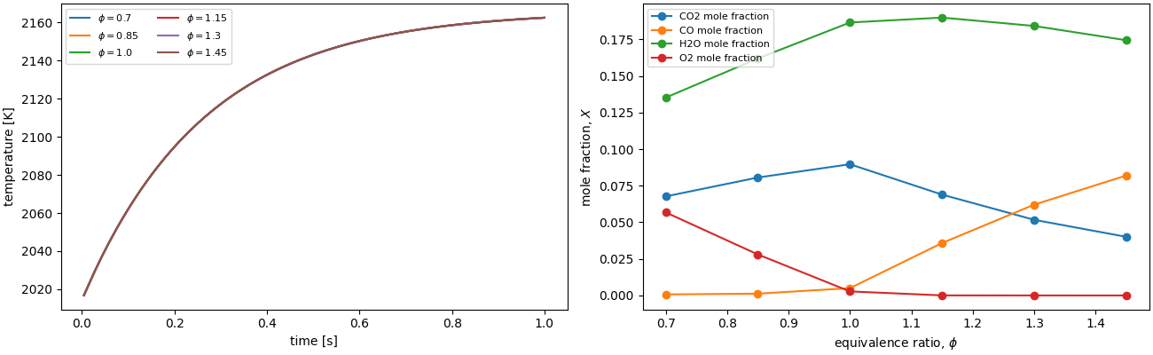
All four configurations produce essentially the same results; the plot shows the results from the fully preconditioned solve. The left panel shows the strong wall coupling pulling the sectors to a nearly common temperature that asymptotically rises as the network approaches steady operation. The right panel shows that the chemistry stays distinct between sectors: CO₂ peaks near the stoichiometric point (\(\phi = 1\)) and falls off on either side, while CO is essentially absent in the lean sectors and accumulates monotonically in the rich sectors.
fig, (ax_T, ax_X) = plt.subplots(1, 2, figsize=(13, 4))
phi_labels = [rf"$\phi = {phi}$" for phi in EQUIVALENCE_RATIOS]
for i in range(len(EQUIVALENCE_RATIOS)):
    ax_T.plot(full["states"][i].t, full["states"][i].T, label=phi_labels[i])
ax_T.set(xlabel="time [s]", ylabel="temperature [K]")
ax_T.legend(fontsize=8, ncol=2)

for species in ("CO2", "CO", "H2O", "O2"):
    X = [states(species).X[-1] for states in full["states"]]
    ax_X.plot(EQUIVALENCE_RATIOS, X, "o-", label=f"{species} mole fraction")
ax_X.set(xlabel=r"equivalence ratio, $\phi$", ylabel="mole fraction, $X$")
ax_X.legend(fontsize=8)
plt.show()
Total running time of the script: (0 minutes 7.198 seconds)