
Note
Go to the end to download the full example code.
Interactive Reaction Path Diagrams#
This example uses ipywidgets to create interactive displays of reaction path
diagrams from Cantera simulations.
Requires: cantera >= 3.0.0, matplotlib >= 2.0, ipywidgets, graphviz, scipy
Tip
To try the interactive features, download the Jupyter notebook version of this
example: interactive_path_diagram.ipynb.
import numpy as np
from scipy import integrate
import graphviz
import os
from matplotlib import pyplot as plt
from collections import defaultdict
import cantera as ct

print(f"Using Cantera version: {ct.__version__}")

# Determine if we're running in a Jupyter Notebook. If so, we can enable the interactive
# diagrams. Otherwise, just draw output for a single set of inputs.
try:
    from IPython import get_ipython
    if "IPKernelApp" not in get_ipython().config:
        raise ImportError("console")
    if "VSCODE_PID" in os.environ:
        raise ImportError("vscode")
except (ImportError, AttributeError):
    is_interactive = False
else:
    is_interactive = True

if is_interactive:
    from IPython.display import display
    from matplotlib_inline.backend_inline import set_matplotlib_formats
    set_matplotlib_formats('pdf', 'svg')
    from ipywidgets import widgets, interact
Using Cantera version: 3.1.0a2
When using Cantera, the first thing you usually need is an object representing some phase of matter. Here, we’ll create a gas mixture using GRI-Mech:
gas = ct.Solution("gri30.yaml")
Use Shock tube ignition delay measurement conditions corresponding to the experiments by Spadaccini and Colket [1].
CH₄-C₂H₆-O₂-Ar (3.29%-0.21%-7%-89.5%)
\(\phi\) = 1.045
P = 6.1 - 7.6 atm
T = 1356 - 1688 K
# Set temperature, pressure, and composition
gas.TPX = 1550.0, 6.5 * ct.one_atm, "CH4:3.29, C2H6:0.21, O2:7 , Ar:89.5"
Residence time is close to ignition delay reported by Spadaccini and Colket (1994).
residence_time = 1e-3
Create a batch reactor object and set solver tolerances
reactor = ct.IdealGasConstPressureReactor(gas, energy="on")
reactor_network = ct.ReactorNet([reactor])
reactor_network.atol = 1e-12
reactor_network.rtol = 1e-12
Store time, pressure, temperature and mole fractions
Interactive reaction path diagram#
When executed as a Jupyter Notebook, the plotted time step, threshold and element can be changed using the slider provided by IPyWidgets.
def plot_reaction_path_diagrams(plot_step, threshold, details, element):
    P = profiles["pressure"][plot_step]
    T = profiles["temperature"][plot_step]
    X = profiles["mole_fractions"][plot_step]
    time = profiles["time"][plot_step]
    gas.TPX = T, P, X

    diagram = ct.ReactionPathDiagram(gas, element)
    diagram.threshold = threshold
    diagram.title = f"time = {time:.2g} s"

    diagram.show_details = details
    graph = graphviz.Source(diagram.get_dot())
    if is_interactive:
        display(graph)
    else:
        return graph

if is_interactive:
    interact(
        plot_reaction_path_diagrams,
        plot_step=widgets.IntSlider(value=100, min=0, max=steps-1, step=10),
        threshold=widgets.FloatSlider(value=0.1, min=0.001, max=0.4, step=0.01),
        details=widgets.ToggleButton(),
        element=widgets.Dropdown(
            options=gas.element_names,
            value="C",
            description="Element",
            disabled=False,
        ),
    )
else:
    # For non-interactive use, just draw the diagram for a specified time step
    diagram = plot_reaction_path_diagrams(
        plot_step=100,
        threshold=0.1,
        details=False,
        element="C"
    )

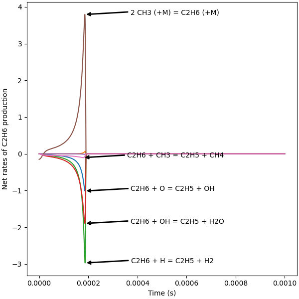
Interactive plot of instantaneous fluxes#
Find reactions containing the species of interest, C₂H₆ in this case.
C2H6_stoichiometry = np.zeros_like(gas.reactions())
for i, r in enumerate(gas.reactions()):
    C2H6_moles = r.products.get("C2H6", 0) - r.reactants.get("C2H6", 0)
    C2H6_stoichiometry[i] = C2H6_moles
C2H6_reaction_indices = C2H6_stoichiometry.nonzero()[0]
The following cell calculates net rates of progress of reactions containing the species of interest and stores them.
profiles["C2H6_production_rates"] = []
for i in range(len(profiles["time"])):
    X = profiles["mole_fractions"][i]
    t = profiles["time"][i]
    T = profiles["temperature"][i]
    P = profiles["pressure"][i]
    gas.TPX = (T, P, X)
    C2H6_production_rates = (
        gas.net_rates_of_progress
        * C2H6_stoichiometry  #  [kmol/m^3/s]
        * gas.volume_mass  # Specific volume [m^3/kg].
    )  # overall, mol/s/g  (g total in reactor, same basis as N_atoms_in_fuel)

    profiles["C2H6_production_rates"].append(
        C2H6_production_rates[C2H6_reaction_indices]
    )

# Create the instantaneous flux plot. When executed as a Jupyter Notebook, the threshold
# for annotating of reaction strings can be changed using the slider provided by
# IPyWidgets.

plt.rcParams["figure.constrained_layout.use"] = True

def plot_instantaneous_fluxes(profiles, annotation_cutoff):
    profiles = profiles
    fig = plt.figure(figsize=(6, 6))
    plt.plot(profiles["time"], np.array(profiles["C2H6_production_rates"]))

    for i, C2H6_production_rate in enumerate(
        np.array(profiles["C2H6_production_rates"]).T
    ):
        peak_index = abs(C2H6_production_rate).argmax()
        peak_time = profiles["time"][peak_index]
        peak_C2H6_production = C2H6_production_rate[peak_index]
        reaction_string = gas.reaction_equations(C2H6_reaction_indices)[i]

        if abs(peak_C2H6_production) > annotation_cutoff:
            plt.annotate(
                reaction_string.replace("<=>", "="),
                xy=(peak_time, peak_C2H6_production),
                xytext=(
                    peak_time * 2,
                    (
                        peak_C2H6_production
                        + 0.003
                        * (peak_C2H6_production / abs(peak_C2H6_production))
                        * (abs(peak_C2H6_production) > 0.005)
                        * (peak_C2H6_production < 0.06)
                    ),
                ),
                arrowprops=dict(
                    arrowstyle="->",
                    color="black",
                    relpos=(0, 0.6),
                    linewidth=2,
                ),
                horizontalalignment="left",
            )

    plt.xlabel("Time (s)")
    plt.ylabel("Net rates of C2H6 production")
    plt.show()

if is_interactive:
    interact(
        plot_instantaneous_fluxes,
        annotation_cutoff=widgets.FloatSlider(value=0.1, min=1e-2, max=4, steps=10),
        profiles=widgets.fixed(profiles)
    )
else:
    plot_instantaneous_fluxes(annotation_cutoff=0.1, profiles=profiles)
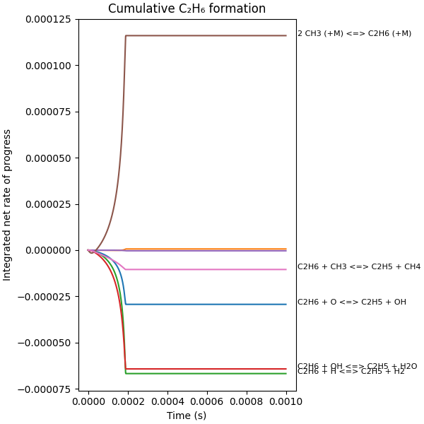
Interactive plot of integrated fluxes#
When executed as a Jupyter Notebook, the threshold for annotating of reaction strings can be changed using the slider provided by iPyWidgets
# Integrate fluxes over time
integrated_fluxes = integrate.cumulative_trapezoid(
    np.array(profiles["C2H6_production_rates"]),
    np.array(profiles["time"]),
    axis=0,
    initial=0,
)

def plot_integrated_fluxes(profiles, integrated_fluxes, annotation_cutoff):
    profiles = profiles
    integrated_fluxes = integrated_fluxes
    fig = plt.figure(figsize=(6, 6))
    plt.plot(profiles["time"], integrated_fluxes)
    final_time = profiles["time"][-1]
    for i, C2H6_production in enumerate(integrated_fluxes.T):
        total_C2H6_production = C2H6_production[-1]
        reaction_string = gas.reaction_equations(C2H6_reaction_indices)[i]

        if abs(total_C2H6_production) > annotation_cutoff:
            plt.text(final_time * 1.06, total_C2H6_production, reaction_string,
                     fontsize=8)

    plt.xlabel("Time (s)")
    plt.ylabel("Integrated net rate of progress")
    plt.title("Cumulative C₂H₆ formation")
    plt.show()

if is_interactive:
    interact(
        plot_integrated_fluxes,
        annotation_cutoff=widgets.FloatLogSlider(
            value=1e-5, min=-5, max=-4, base=10, step=0.1
        ),
        profiles=widgets.fixed(profiles),
        integrated_fluxes=widgets.fixed(integrated_fluxes)
    )
else:
    plot_integrated_fluxes(
        profiles=profiles,
        integrated_fluxes=integrated_fluxes,
        annotation_cutoff=1e-5
    )
References#
Total running time of the script: (0 minutes 0.773 seconds)