Reactors with walls and heat transfer#

Two reactors connected with a piston, with heat loss to the environment

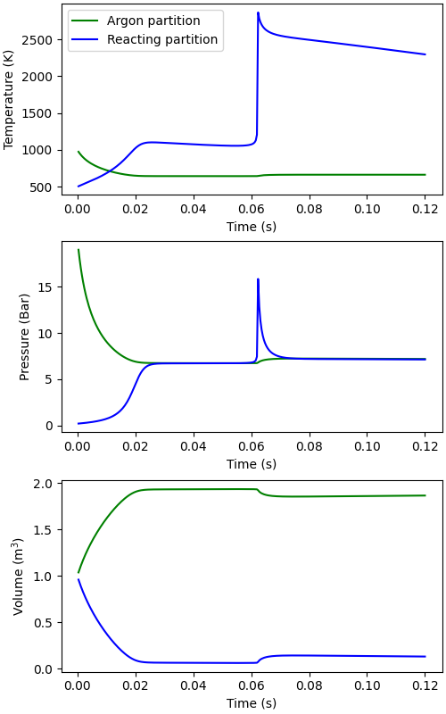
This script simulates the following situation. A closed cylinder with volume 2 m³ is divided into two equal parts by a massless piston that moves with speed proportional to the pressure difference between the two sides. It is initially held in place in the middle. One side is filled with 1000 K argon at 20 atm, and the other with a combustible 500 K methane/air mixture at 0.2 atm ( $ϕ = 1.1$ ). At $t = 0$ , the piston is released and begins to move due to the large pressure difference, compressing and heating the methane/air mixture, which eventually explodes. At the same time, the argon cools as it expands. The piston allows heat transfer between the reactors and some heat is lost through the outer cylinder walls to the environment.

Note that this simulation, being zero-dimensional, takes no account of shock wave propagation. It is somewhat artificial, but nevertheless instructive.

Requires: cantera >= 2.5.0, matplotlib >= 2.0, pandas

Tags: combustion reactor network plotting

import pandas as pd
import matplotlib.pyplot as plt
plt.rcParams['figure.constrained_layout.use'] = True

import cantera as ct

Set up the simulation#

First create each gas needed, and a reactor or reservoir for each one.

# create an argon gas object and set its state
ar = ct.Solution('air.yaml')
ar.TPX = 1000.0, 20.0 * ct.one_atm, "AR:1"

# create a reactor to represent the side of the cylinder filled with argon
r1 = ct.IdealGasReactor(ar, name="Argon partition")

# create a reservoir for the environment, and fill it with air.
env = ct.Reservoir(ct.Solution('air.yaml'), name="Environment")

# use GRI-Mech 3.0 for the methane/air mixture, and set its initial state
gas = ct.Solution('gri30.yaml')
gas.TP = 500.0, 0.2 * ct.one_atm
gas.set_equivalence_ratio(1.1, 'CH4:1.0', 'O2:1, N2:3.76')

# create a reactor for the methane/air side
r2 = ct.IdealGasReactor(gas, name="Reacting partition")

# Now couple the reactors by defining common walls that may move (a piston) or
# conduct heat

# add a flexible wall (a piston) between r2 and r1
w = ct.Wall(r2, r1, A=1.0, K=0.5e-4, U=100.0, name="Piston")

# heat loss to the environment. Heat loss always occur through walls, so we
# create a wall separating r2 from the environment, give it a non-zero area,
# and specify the overall heat transfer coefficient through the wall.
w2 = ct.Wall(r2, env, A=1.0, U=500.0, name="External Wall")

sim = ct.ReactorNet([r1, r2])

Show the initial state#

sim.draw(print_state=True, species="X")

Now the problem is set up, and we’re ready to solve it.

time = 0.0
n_steps = 300
states1 = ct.SolutionArray(ar, extra=['t', 'V'])
states2 = ct.SolutionArray(gas, extra=['t', 'V'])

for n in range(n_steps):
    time += 4.e-4
    sim.advance(time)
    states1.append(r1.thermo.state, t=time, V=r1.volume)
    states2.append(r2.thermo.state, t=time, V=r2.volume)

Combine the results and save for later processing or plotting

df = pd.DataFrame.from_dict({
    'time (s)': states1.t,
    'T1 (K)': states1.T,
    'P1 (bar)': states1.P / 1e5,
    'V1 (m3)': states1.V,
    'T2 (K)': states2.T,
    'P2 (bar)': states2.P / 1e5,
    'V2 (m3)': states2.V,
})
df.to_csv("piston.csv")
df

	time (s)	T1 (K)	P1 (bar)	V1 (m3)	T2 (K)	P2 (bar)	V2 (m3)
0	0.0004	974.915404	19.018144	1.038832	506.904245	0.213749	0.961168
1	0.0008	952.717786	17.954178	1.075339	513.699629	0.225166	0.924661
2	0.0012	932.862197	17.033443	1.109843	520.417757	0.236953	0.890157
3	0.0016	914.941012	16.227259	1.142601	527.084726	0.249158	0.857399
4	0.0020	898.641990	15.514320	1.173817	533.722660	0.261828	0.826183
...	...	...	...	...	...	...	...
295	0.1184	663.499539	7.202775	1.866755	2303.353984	7.147006	0.133245
296	0.1188	663.494672	7.202292	1.866867	2301.302242	7.146505	0.133133
297	0.1192	663.489772	7.201808	1.866978	2299.249665	7.146005	0.133022
298	0.1196	663.484838	7.201324	1.867090	2297.196284	7.145504	0.132910
299	0.1200	663.479871	7.200840	1.867202	2295.142132	7.145004	0.132798

300 rows × 7 columns

Plot results#

fig, ax = plt.subplots(3, 1, figsize=(5,8))

ax[0].plot(states1.t, states1.T, 'g-', label='Argon partition')
ax[0].plot(states2.t, states2.T, 'b-', label='Reacting partition')
ax[0].set(xlabel='Time (s)', ylabel='Temperature (K)')
ax[0].legend()

ax[1].plot(states1.t, states1.P / 1e5, 'g-', states2.t, states2.P / 1e5, 'b-')
ax[1].set(xlabel='Time (s)', ylabel='Pressure (Bar)')

ax[2].plot(states1.t, states1.V, 'g-', states2.t, states2.V, 'b-')
_ = ax[2].set(xlabel='Time (s)', ylabel='Volume (m$^3$)')

Show the final state#

try:
    diagram = sim.draw(print_state=True, species="X")
except ImportError as err:
    print(f"Unable to show network structure:\n{err}")

Total running time of the script: (0 minutes 0.690 seconds)

Gallery generated by Sphinx-Gallery