Note

Go to the end to download the full example code.

One-dimensional packed-bed, catalytic-membrane reactor#

The model shown in this example simulates heterogeneous catalytic processes inside packed-bed, catalytic membrane reactors. The gas-phase and surface-phase species conservation equations are derived and the system of differential-algebraic equations (DAE) is solved using the scikits.odes.dae IDA solver.

Requires: cantera >= 3.0.0, matplotlib >= 2.0, scikits.odes >= 2.7.0

Tags: Python surface chemistry 1D flow catalysis packed bed reactor porous media user-defined model

Methodology#

A one-dimensional, steady-state catalytic-membrane reactor model with surface chemistry is developed to analyze species profiles along the length of a packed-bed, catalytic membrane reactor. The same model can further be simplified to simulate a simple packed-bed reactor by excluding the membrane. The example here demonstrates the one-dimensional reactor model explained by G. Kogekar [1].

Governing equations#

Assuming steady-state, one-dimensional flow within the packed bed, total-mass, species mass and energy conservation may be stated as [2]:

\begin{array}{r} \begin{aligned} \begin{aligned} \frac{d (ρ u)}{d z} & = \sum_{k = 1}^{K_{g}} {\dot{s}}_{k} W_{k} A_{s} + \frac{P_{b}}{A_{b}} j_{k_{M}}, \end{aligned} \\ \begin{aligned} ρ u \frac{d Y_{k}}{d z} + A_{s} Y_{k} \sum_{k = 1}^{K_{g}} {\dot{s}}_{k} W_{k} & = A_{s} {\dot{s}}_{k} W_{k} + δ_{k, k_{M}} \frac{P_{b}}{A_{b}} j_{k_{M}}, \end{aligned} \\ ρ u c_{p} \frac{d T}{d z} + \sum_{k = 1}^{K_{g}} h_{k} (ϕ_{g} {\dot{ω}}_{k} + A_{s} {\dot{s}}_{k}) W_{k} & = \hat{h} \frac{P_{b}}{A_{b}} (T_{w} - T) + δ_{k, k_{M}} \frac{P_{b}}{A_{b}} h_{k_{M}} j_{k_{M}} . \end{aligned} \end{array}

The fractional coverages of the $K_{s}$ surface adsorbates $θ_{k}$ must satisfy

{\dot{s}}_{k} = 0, (k = 1, \dots, K_{s}),

which, at steady state, requires no net production/consumption of surface species by the heterogeneous reactions [3].

The pressure within the bed is calculated as:

\frac{d p}{d z} = - (\frac{ϕ_{g} μ}{β_{g}}) u,

where $μ$ is the gas-phase mixture viscosity. The packed-bed permeability :math:beta_t{g}` is evaluated using the Kozeny-Carman relationship as

β_{g} = \frac{ϕ_{g}^{3} D_{p}^{2}}{72 τ_{g} (1 - ϕ_{g})^{2}},

where $ϕ_{g}$ , $τ_{g}$ , and $D_{p}$ are the bed porosity, tortuosity, and particle diameter, respectively.

The independent variable in these conservation equations is the position $z$ along the reactor length. The dependent variables include total mass flux $ρ u$ , pressure $p$ , temperature $T$ , gas-phase mass fractions $Y_{k}$ , and surfaces coverages $θ_{k}$ . Gas-phase fluxes through the membrane are represented as $j_{k, M}$ . Geometric parameters $A_{s}$ , $P_{b}$ , and $A_{b}$ represent the catalyst specific surface area (dimensions of surface area per unit volume), reactor perimeter, and reactor cross-sectional flow area, respectively. Other parameters include bed porosity $ϕ_{g}$ and gas-phase species molecular weights $W_{k}$ . The gas density $ρ$ is evaluated using the equation of state (such as ideal gas, Redlich-Kwong or Peng-Robinson).

If a perm-selective membrane is present, then $j_{k_{M}}$ represents the gas-phase flux through the membrane and $k_{M}$ is the gas-phase species that permeates through the membrane. The Kronecker delta, $δ_{k, k_{M}} = 1$ for the membrane-permeable species and $δ_{k, k_{M}} = 0$ otherwise. The membrane flux is calculated using Sievert’s law as

j_{k_{M}}^{Mem} = \frac{B_{k_{M}}}{t} (p_{k_{M}, mem}^{α} - p_{k_{M}, sweep}^{α}) W_{k_{M}}

where $B_{k_{M}}$ is the membrane permeability, $t$ is the membrane thickness. $p_{k_{M}, mem}$ and $p_{k_{M}, sweep}$ represent perm-selective species partial pressures within the packed-bed and the exterior sweep channel. The present model takes the pressure exponent $α$ to be unity. The membrane flux for all other species ( $k \neq k_{M}$ ) is zero.

Chemistry mechanism#

This example uses a detailed 12-step elementary micro-kinetic reaction mechanism that describes ammonia formation and decomposition kinetics over the Ru/Ba-YSZ catalyst. The reaction mechanism is developed and validated using measured performance in a laboratory-scale packed-bed reactor [4]. This example also incorporates a Pd-based H₂ perm-selective membrane.

Solver#

The above governing equations represent a complete solution for a steady-state packed-bed, catalytic membrane reactor model. The dependent variables are the mass-flux $ρ u$ , species mass-fractions $Y_{k}$ , pressure $p$ , temperature $T$ , and surface coverages $θ_{k}$ . The equation of state is used to obtain the mass density, $ρ$ .

The governing equations form an initial value problem (IVP) in a differential-algebraic (DAE) form as follows:

f (z, y, y^{'}, c) = 0,

where $y$ and $y^{'}$ represent the state vector and its derivative vector, respectively. All other constants such as reference temperature, chemical constants, etc. are incorporated in vector $c$ (Refer to [1] for more details). This type of DAE system in this example is solved using the scikits.odes.dae IDA solver.

Import Cantera and scikits#

import numpy as np
from scikits.odes import dae
import cantera as ct
import matplotlib.pyplot as plt

Define gas-phase and surface-phase species#

# Import the reaction mechanism for Ammonia synthesis/decomposition on Ru-Ba/YSZ catalyst
mechfile = "example_data/ammonia-Ru-Ba-YSZ-CSM-2019.yaml"
# Import the models for surface-phase and gas
surf = ct.Interface(mechfile, "Ru_surface")
gas = surf.adjacent["gas"]

# Other parameters
n_gas = gas.n_species  # number of gas species
n_surf = surf.n_species  # number of surface species
n_gas_reactions = gas.n_reactions  # number of gas-phase reactions

# Set offsets of dependent variables in the solution vector
offset_rhou = 0
offset_p = 1
offset_T = 2
offset_Y = 3
offset_Z = offset_Y + n_gas
n_var = offset_Z + n_surf  # total number of variables (rhou, P, T, Yk and Zk)

print("Number of gas-phase species = ", n_gas)
print("Number of surface-phase species = ", n_surf)
print("Number of variables = ", n_var)

Number of gas-phase species =  4
Number of surface-phase species =  6
Number of variables =  13

Define reactor geometry and operating conditions#

# Reactor geometry
L = 5e-2  # length of the reactor (m)
R = 5e-3  # radius of the reactor channel (m)
phi = 0.5  # porosity of the bed (-)
tau = 2.0  # tortuosity of the bed (-)
dp = 3.37e-4  # particle diameter (m)
As = 3.5e6  # specific surface area (1/m)

# Energy (adiabatic or isothermal)
solve_energy = True  # True: Adiabatic, False: isothermal

# Membrane (True: membrane, False: no membrane)
membrane_present = True
membrane_perm = 1e-15  # membrane permeability (kmol*m3/s/Pa)
thickness = 3e-6  # membrane thickness (m)
membrane_sp_name = "H2"  # membrane-permeable species name
p_sweep = 1e5  # partial pressure of permeable species in the sweep channel (Pa)
permeance = membrane_perm / thickness  # permeance of the membrane (kmol*m2/s/Pa)

if membrane_present:
    print("Modeling packed-bed, catalytic-membrane reactor...")
    print(membrane_sp_name, "permeable membrane is present.")

# Get required properties based on the geometry and mechanism
W_g = gas.molecular_weights  # vector of molecular weight of gas species
vol_ratio = phi / (1 - phi)
eff_factor = phi / tau  # effective factor for permeability calculation
# permeability based on Kozeny-Carman equation
B_g = B_g = vol_ratio**2 * dp**2 * eff_factor / 72
area2vol = 2 / R  # area to volume ratio assuming a cylindrical reactor
D_h = 2 * R  # hydraulic diameter
membrane_sp_ind = gas.species_index(membrane_sp_name)

# Inlet operating conditions
T_in = 673  # inlet temperature [K]
p_in = 5e5  # inlet pressure [Pa]
v_in = 0.001  # inlet velocity [m/s]
T_wall = 723  # wall temperature [K]
h_coeff = 1e2  # heat transfer coefficient [W/m2/K]

# Set gas and surface states
gas.TPX = T_in, p_in, "NH3:0.99, AR:0.01"  # inlet composition
surf.TP = T_in, p_in
Yk_0 = gas.Y
rhou0 = gas.density * v_in

# Initial surface coverages
# advancing coverages over a long period of time to get the steady state.
surf.advance_coverages(1e10)
Zk_0 = surf.coverages

Modeling packed-bed, catalytic-membrane reactor...
H2 permeable membrane is present.

Define residual function required for IDA solver#

def residual(z, y, yPrime, res):
    """Solution vector for the model
    y = [rho*u, p, T, Yk, Zk]
    yPrime = [d(rho*u)dz, dpdz, dTdz, dYkdz, dZkdz]
    """
    # Get current thermodynamic state from solution vector and save it to local variables.
    rhou = y[offset_rhou]  # mass flux (density * velocity)
    Y = y[offset_Y : offset_Y + n_gas]  # vector of mass fractions
    Z = y[offset_Z : offset_Z + n_surf] # vector of site fractions
    p = y[offset_p]  # pressure
    T = y[offset_T]  # temperature

    # Get derivatives of dependent variables
    drhoudz = yPrime[offset_rhou]
    dYdz = yPrime[offset_Y : offset_Y + n_gas]
    dZdz = yPrime[offset_Z : offset_Z + n_surf]
    dpdz = yPrime[offset_p]
    dTdz = yPrime[offset_T]

    # Set current thermodynamic state for the gas and surface phases
    # Note: use unnormalized mass fractions and site fractions to avoid
    # over-constraining the system
    gas.set_unnormalized_mass_fractions(Y)
    gas.TP = T, p
    surf.set_unnormalized_coverages(Z)
    surf.TP = T, p

    # Calculate required variables based on the current state
    coverages = surf.coverages  # surface site coverages
    # heterogeneous production rate of gas species
    sdot_g = surf.get_net_production_rates("gas")
    # heterogeneous production rate of surface species
    sdot_s = surf.get_net_production_rates("Ru_surface")
    wdot_g = np.zeros(n_gas)
    # specific heat of the mixture
    cp = gas.cp_mass
    # partial enthalpies of gas species
    hk_g = gas.partial_molar_enthalpies

    if n_gas_reactions > 0:
        # homogeneous production rate of gas species
        wdot_g = gas.net_production_rates
    mu = gas.viscosity  # viscosity of the gas-phase

    # Calculate density using equation of state
    rho = gas.density

    # Calculate flux term through the membrane
    # partial pressure of membrane-permeable species
    memsp_pres = p * gas.X[membrane_sp_ind]
    # negative sign indicates the flux going out
    membrane_flux = -permeance * (memsp_pres - p_sweep) * W_g[membrane_sp_ind]

    # Conservation of total-mass
    # temporary variable
    sum_continuity = As * np.sum(sdot_g * W_g) + phi * np.sum(wdot_g * W_g)
    res[offset_rhou] = (drhoudz - sum_continuity
                        - area2vol * membrane_flux * membrane_present)

    # Conservation of gas-phase species
    res[offset_Y:offset_Y+ n_gas] = (dYdz + (Y * sum_continuity
                                             - phi * np.multiply(wdot_g,W_g)
                                             - As * np.multiply(sdot_g,W_g)) / rhou)
    res[offset_Y + membrane_sp_ind] -= area2vol * membrane_flux * membrane_present

    # Conservation of site fractions (algebraic constraints in this example)
    res[offset_Z : offset_Z + n_surf] = sdot_s

    # For the species with largest site coverage (k_large), solve the constraint
    # equation: sum(Zk) = 1.
    # The residual function for 'k_large' would be 'res[k_large] = 1 - sum(Zk)'
    # Note that here sum(Zk) will be the sum of coverages for all surface species,
    # including the 'k_large' species.
    ind_large = np.argmax(coverages)
    res[offset_Z + ind_large] = 1 - np.sum(coverages)

    # Conservation of momentum
    u = rhou / rho
    res[offset_p] = dpdz + phi * mu * u / B_g

    # Conservation of energy
    res[offset_T] = dTdz - 0  # isothermal condition
    # Note: One can just not solve the energy equation by keeping temperature constant.
    # But since 'T' is used as the dependent variable, the residual is res[T] = dTdz - 0
    # One can also write res[T] = 0 directly, but that leads to a solver failure due to
    # singular jacobian

    if solve_energy:
        conv_term = (4 / D_h) * h_coeff * (T_wall - T) * (2 * np.pi * R)
        chem_term = np.sum(hk_g * (phi * wdot_g + As * sdot_g))
        res[offset_T] -= (conv_term - chem_term) / (rhou * cp)

Calculate the spatial derivatives at the inlet that will be used as the initial conditions for the IDA solver

# Initialize yPrime to 0 and call residual to get initial derivatives
y0 = np.hstack((rhou0, p_in, T_in, Yk_0, Zk_0))
yprime0 = np.zeros(n_var)
res = np.zeros(n_var)
residual(0, y0, yprime0, res)
yprime0 = -res

Solve the system of DAEs using IDA solver#

solver = dae(
    "ida",
    residual,
    first_step_size=1e-15,
    atol=1e-14,  # absolute tolerance for solution
    rtol=1e-06,  # relative tolerance for solution
    algebraic_vars_idx=[np.arange(offset_Y + n_gas, offset_Z + n_surf, 1)],
    max_steps=8000,
    one_step_compute=True,
    old_api=False,  # forces use of new api (namedtuple)
)

distance = []
solution = []
state = solver.init_step(0.0, y0, yprime0)

# Note that here the variable t is an internal variable used in scikits. In this
# example, it represents the natural variable z, which corresponds to the axial distance
# inside the reactor.
while state.values.t < L:
    distance.append(state.values.t)
    solution.append(state.values.y)
    state = solver.step(L)

distance = np.array(distance)
solution = np.array(solution)
print(state)

SolverReturn(flag=<StatusEnumIDA.SUCCESS: 0>, values=SolverVariables(t=0.05023281932803743, y=array([1.07319177e-03, 4.99997967e+05, 6.85046104e+02, 8.79760300e-02,
       4.78735832e-01, 4.09673345e-01, 2.31456973e-02, 3.26039256e-03,
       9.93142959e-01, 2.67802570e-03, 8.56453407e-04, 3.65354138e-08,
       6.21324677e-05]), ydot=array([-4.05716608e-02, -3.51713818e+01,  3.08767242e+01,  2.51631585e+00,
       -1.44016568e+01,  1.18447750e+01, -5.35520657e-06,  2.12651775e-01,
       -4.20589590e-01,  1.99058511e-01,  7.32611506e-03,  6.31495314e-07,
        1.55255724e-03])), errors=SolverVariables(t=None, y=None, ydot=None), roots=SolverVariables(t=None, y=None, ydot=None), tstop=SolverVariables(t=None, y=None, ydot=None), message='Successful function return.')

Plot results#

plt.rcParams['figure.constrained_layout.use'] = True

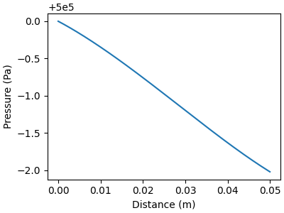
Pressure and temperature#

# Plot gas pressure profile along the flow direction
f, ax = plt.subplots(figsize=(4,3))
ax.plot(distance, solution[:, offset_p], color="C0")
ax.set_xlabel("Distance (m)")
ax.set_ylabel("Pressure (Pa)")

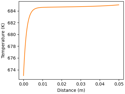
# Plot gas temperature profile along the flow direction
f, ax = plt.subplots(figsize=(4,3))
ax.plot(distance, solution[:, offset_T], color="C1")
ax.set_xlabel("Distance (m)")
ax.set_ylabel("Temperature (K)")

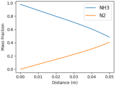
Mass fractions of the gas-phase species#

# Plot major and minor gas species separately
minor_idx = []
major_idx = []
for j, name in enumerate(gas.species_names):
    mean = np.mean(solution[:, offset_Y + j])
    if mean <= 0.1:
        minor_idx.append(j)
    else:
        major_idx.append(j)

# Major gas-phase species
f, ax = plt.subplots(figsize=(4,3))
for j in major_idx:
    ax.plot(distance, solution[:, offset_Y + j], label=gas.species_names[j])
ax.legend(fontsize=12, loc="best")
ax.set_xlabel("Distance (m)")
ax.set_ylabel("Mass Fraction")

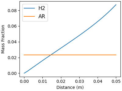
# Minor gas-phase species
f, ax = plt.subplots(figsize=(4,3))
for j in minor_idx:
    ax.plot(distance, solution[:, offset_Y + j], label=gas.species_names[j])
ax.legend(fontsize=12, loc="best")
ax.set_xlabel("Distance (m)")
ax.set_ylabel("Mass Fraction")

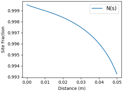
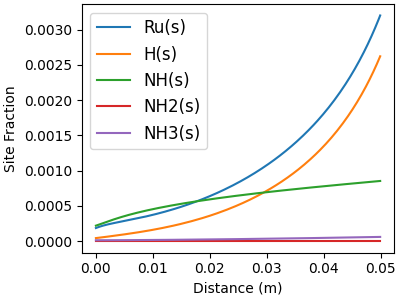
Site fractions of the surface-phase species#

# Plot major and minor surface species separately
minor_idx = []
major_idx = []
for j, name in enumerate(surf.species_names):
    mean = np.mean(solution[:, offset_Z + j])
    if mean <= 0.1:
        minor_idx.append(j)
    else:
        major_idx.append(j)

# Major surf-phase species
f, ax = plt.subplots(figsize=(4,3))
for j in major_idx:
    ax.plot(distance, solution[:, offset_Z + j], label=surf.species_names[j])
ax.legend(fontsize=12, loc="best")
ax.set_xlabel("Distance (m)")
ax.set_ylabel("Site Fraction")

# Minor surf-phase species
f, ax = plt.subplots(figsize=(4,3))
for j in minor_idx:
    ax.plot(distance, solution[:, offset_Z + j], label=surf.species_names[j])
ax.legend(fontsize=12, loc="best")
ax.set_xlabel("Distance (m)")
ax.set_ylabel("Site Fraction")

References#

Total running time of the script: (0 minutes 0.948 seconds)

Gallery generated by Sphinx-Gallery