Lithium Ion Battery Discharge Curve#

Kinetic equilibrium calculations#

In the kinetic equilibrium problem, steady state is achieved when the faradaic current at each electrode (anode and cathode) surface and the ionic current through the electrolyte are all zero. There are, essentially, four relevant electric potentials which must be determined:

• ${\varphi }_{\mathrm{a}\mathrm{n}\mathrm{o}\mathrm{d}\mathrm{e}}$: electric potential of graphite anode.

• ${\varphi }_{\mathrm{e}\mathrm{l}\mathrm{y}\mathrm{t}\mathrm{e},\mathrm{a}\mathrm{n}\mathrm{o}\mathrm{d}\mathrm{e}}$: electric potential of electrolyte at anode interface.

• ${\varphi }_{\mathrm{e}\mathrm{l}\mathrm{y}\mathrm{t}\mathrm{e},\mathrm{c}\mathrm{a}\mathrm{t}\mathrm{h}\mathrm{o}\mathrm{d}\mathrm{e}}$: electric potential of electrolyte at cathode interface.

• ${\varphi }_{\mathrm{c}\mathrm{a}\mathrm{t}\mathrm{h}\mathrm{o}\mathrm{d}\mathrm{e}}$: electric potential of LCO cathode.

Setting one of these four to the reference potential of zero (because it is the difference in electric potential which drives currents, the actual potential values are irrelevant. Let’s assume the anode electric potential is zero), there is only one distribution of electric potentials across the cell such that the current is invariant across the cell. I.e. we want the potentials such that:

where $i_{\mathrm{a}\mathrm{p}\mathrm{p}}$ is the user input for the applied current. For this example, we assume an applied current of 0, to calculate the equilibrium voltage.

import numpy as np
from scipy.optimize import fsolve
import time  # Used for timing our calculations
import matplotlib.pyplot as plt
import cantera as ct
print(f"Runnning Cantera version: {ct.__version__}")

Runnning Cantera version: 3.1.0

Define the phases#

The phase thermodynamics are defined according to experimentally-measured open circuit voltage values, as described in the reference provided above. These values are stored in the input file lithium_ion_battery.yaml.

input_file = "../data/lithium_ion_battery.yaml"
anode = ct.Solution(input_file, "anode")
cathode = ct.Solution(input_file, "cathode")
# The 'elde' electrode phase is needed as a source/sink for electron
elde = ct.Solution(input_file, "electron")
elyte = ct.Solution(input_file, "electrolyte")
anode_interface = ct.Interface(
    input_file, "edge_anode_electrolyte", [anode, elde, elyte]
)
cathode_interface = ct.Interface(
    input_file, "edge_cathode_electrolyte", [cathode, elde, elyte]
)

Define battery conditions: temperature, pressure, stoichiometry, electrolyte resistance#

Inputs are:

• Stoichiometries X_Li_ca and X_Li_an [-] (can be vectors)

• Temperature T [K]

• Pressure P [Pa]

• Externally-applied current i_app [A]

• Electrolyte resistance R_elyte [Ohm]

• Anode total surface area S_an [m^2]

• Cathode total surface area S_ca [m^2]

# Array of lithium mole fractions in the anode
X_Li_an = np.arange(0.005, 0.995, 0.02)
# Assume that the cathode and anode capacities are balanced
X_Li_ca = 1.0 - X_Li_an

# I_app = 0: Open circuit
I_app = 0.0

# At zero current, electrolyte resistance is irrelevant
R_elyte = 0.0

# Temperature and pressure
T = 300  # K
P = ct.one_atm

F = ct.faraday

# [m^2] Cathode total active material surface area
S_ca = 1.1167

S_an = 0.7824  # [m^2] Anode total active material surface area

Set phase temperatures and pressures#

phases = [anode, elde, elyte, cathode, anode_interface, cathode_interface]
for ph in phases:
    ph.TP = T, P

Helper Functions#

def anode_curr(phi_l, I_app, phi_s, X_Li_an):
    # Set the active material mole fraction
    anode.X = {"Li[anode]": X_Li_an, "V[anode]": 1 - X_Li_an}

    # Set the electrode and electrolyte potential
    elde.electric_potential = phi_s
    elyte.electric_potential = phi_l[0]

    # Get the net product rate of electrons in the anode (per m2^ interface)
    r_elec = anode_interface.get_net_production_rates(elde)

    anode_current = r_elec * ct.faraday * S_an
    diff = I_app + anode_current

    return diff


def cathode_curr(phi_s, I_app, phi_l, X_Li_ca):
    # Set the active material mole fractions
    cathode.X = {"Li[cathode]": X_Li_ca, "V[cathode]": 1 - X_Li_ca}

    # Set the electrode and electrolyte potential
    elde.electric_potential = phi_s[0]
    elyte.electric_potential = phi_l

    # Get the net product rate of electrons in the cathode (per m2^ interface)
    r_elec = cathode_interface.get_net_production_rates(elde)

    cathode_current = r_elec * ct.faraday * S_an
    diff = I_app - cathode_current

    return diff

Run the calculations for all stoichiometries#

# Tic
t0 = time.time()

# Initialize array of OCVs
E_cell_kin = np.zeros_like(X_Li_ca)

for i, X_an in enumerate(X_Li_an):
    # Set anode electrode potential to 0
    phi_s_an = 0
    E_init = 3.0

    phi_l_an = fsolve(anode_curr, E_init, args=(I_app, phi_s_an, X_an))

    # Calculate electrolyte potential at cathode interface
    phi_l_ca = phi_l_an[0] + I_app * R_elyte

    # Calculate cathode electrode potential
    phi_s_ca = fsolve(cathode_curr, E_init, args=(I_app, phi_l_ca, X_Li_ca[i]))

    # Calculate cell voltage
    E_cell_kin[i] = phi_s_ca[0] - phi_s_an

# Toc
t1 = time.time()
print(f"{i:d} cell voltages calculated in {t1 - t0:3.2e} seconds.")

49 cell voltages calculated in 1.74e-02 seconds.

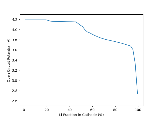
Plot cell voltage, as a function of the cathode stoichiometry#

fig, ax = plt.subplots()
ax.plot(100 * X_Li_ca, E_cell_kin)
_ = ax.set(ylim=[2.5, 4.3], xlabel="Li Fraction in Cathode (%)",
           ylabel="Open Circuit Potential (V)")

Thermodynamic Equilibrium Calculation#

For the $i_{app}=0$ case, we can also calculate the voltage using thermodynamics. At equilibrium, the net electrochemical potential change of the reaction must be zero:

where ${\tilde{\mu }}_k={\mu }_k+z_{k}F{\mathrm{\Phi }}_k$, where, in turn ${\mu }_k=\frac{\partial g_k}{\partial n_k}$ is the chemical potential, ${\nu }_k$ the net stoichiometric coefficient, $z_k$ the net elementary charge, and ${\mathrm{\Phi }}_k$ the phase electric potential for species $k$.

From this, we can calculate the equilibrium electric potential difference $\mathrm{\Delta }{\mathrm{\Phi }}_{\mathrm{e}\mathrm{q}}={({\mathrm{\Phi }}_{\mathrm{e}\mathrm{l}\mathrm{d}\mathrm{e}}-{\mathrm{\Phi }}_{\mathrm{e}\mathrm{l}\mathrm{y}\mathrm{t}\mathrm{e}})}_{\mathrm{e}\mathrm{q}}$ as:

where $\mathrm{\Delta }{g}_{\mathrm{r}\mathrm{x}\mathrm{n}}=\sum _k{\nu }_k{\mu }_k$ is the chemical potential of the reaction and and $n_{\mathrm{c}\mathrm{h}\mathrm{a}\mathrm{r}\mathrm{g}\mathrm{e}}=\sum _{k,\mathrm{e}\mathrm{l}\mathrm{d}\mathrm{e}}{\nu }_k{z}_k$ is the net elementary charge transferred from the electrolyte to the electrode.

# Tic
t0 = time.time()

# Initialize array of OCVs
E_cell_therm = np.zeros_like(X_Li_ca)

for i, X_an in enumerate(X_Li_an):
    # Set anode electrode potential to 0
    anode.X = "Li[anode]:" + str(X_an) + ", V[anode]:" + str(1 - X_an)
    dG_an = anode_interface.delta_gibbs[0]
    n_charge = 1.0
    E_eq_an = -dG_an / n_charge / ct.faraday

    cathode.X = "Li[cathode]:" + str(1.0 - X_an) + ", V[cathode]:" + str(X_an)
    dG_ca = cathode_interface.delta_gibbs[0]
    n_charge = 1.0
    E_eq_ca = -dG_ca / n_charge / ct.faraday

    E_cell_therm[i] = E_eq_ca - E_eq_an

# Toc
t1 = time.time()
print(f"{i:d} cell voltages calculated in {t1 - t0:3.2e} seconds.")

49 cell voltages calculated in 6.53e-04 seconds.

Plot thermodynamic OCV, and compare to results from kinetic method#

fig, ax = plt.subplots()
ax.plot(100 * X_Li_ca, E_cell_kin, label="Kinetic")
ax.plot(100 * X_Li_ca, E_cell_therm,
        linewidth=0.0, marker="o", markerfacecolor="none", label="Thermodynamic")
ax.set(ylim=[2.5, 4.3], xlabel="Li Fraction in Cathode (%)",
       ylabel="Open Circuit Potential (V)")
ax.legend()

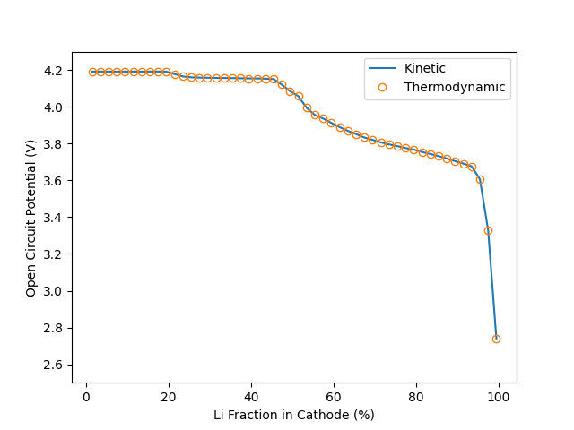
As one would expect, the two approaches give identical results. While both methods are incredibly fast, the thermodynamic method is roughly 30 times faster.

A large part of this is that the thermodynamic approach is an analytical approach (i.e. the answer is known from theory), while the kinetic approach relies on the root-finding fzero method to fit the correct voltage. Note also that the kinetic method, because of the use of Butler-Volmer kinetics, calculates the thermodynamic voltage, in order to calculate the overpotential $\eta =\mathrm{\Delta }\mathrm{\Phi }-\mathrm{\Delta }{\mathrm{\Phi }}_{\mathrm{e}\mathrm{q}}$.

However, it is at last important to note that, while slower, the kinetic method is of course more robust, and can be used to find results away from equilibrium. The thermodynamic method is only applicable at equilibrium (zero current).

Total running time of the script: (0 minutes 0.432 seconds)

Gallery generated by Sphinx-Gallery