Mechanism reduction

A simplistic approach to mechanism reduction which demonstrates Cantera’s features for dynamically manipulating chemical mechanisms.

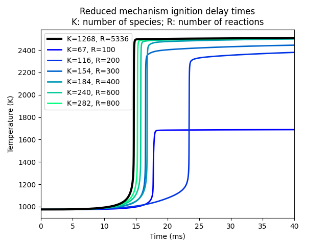
Here, we use the detailed NUI Galway mechanism to simulate adiabatic, constant pressure ignition of a lean n-hexane/air mixture. We track the maximum reaction rates for each reaction to determine which reactions are the most important, according to a simple metric based on the relative net reaction rate.

We then create a sequence of reduced mechanisms including only the top reactions and the associated species, and run the simulations again with these mechanisms to see whether the reduced mechanisms with a certain number of species are able to adequately simulate the ignition delay problem.

Requires: cantera >= 3.1.0, matplotlib >= 2.0

Tags: Python kinetics combustion reactor network editing mechanisms ignition delay plotting

import cantera as ct
import numpy as np
import matplotlib.pyplot as plt
import dataclasses

@dataclasses.dataclass
class Result:
    species: int
    reactions: int
    time: list
    temperature: list


ct.suppress_thermo_warnings()
T0 = 975
P0 = 5 * ct.one_atm
gas = ct.Solution('example_data/n-hexane-NUIG-2015.yaml')
gas.set_equivalence_ratio(0.8, 'NC6H14:1.0', 'O2:1.0, N2:3.76')
X0 = gas.mole_fraction_dict()
gas.TP = T0, P0

Run a simulation with the full mechanism

r = ct.IdealGasConstPressureMoleReactor(gas)
sim = ct.ReactorNet([r])
sim.preconditioner = ct.AdaptivePreconditioner()

tt = []
TT = []
# Rmax is the maximum relative reaction rate at any timestep.
Rmax = np.zeros(gas.n_reactions)
while sim.time < 0.04:
    sim.step()
    tt.append(1000 * sim.time)
    TT.append(r.T)
    rnet = abs(gas.net_rates_of_progress)
    rnet /= max(rnet)
    Rmax = np.maximum(Rmax, rnet)

baseline = Result(gas.n_species, gas.n_reactions, tt, TT)

Get the reaction objects, and sort them so the most active reactions are first.

R = sorted(zip(Rmax, gas.reactions()), key=lambda x: -x[0])

Test reduced mechanisms with different numbers of reactions and collect results for plotting.

results = []
for i, N in enumerate([100, 200, 300, 400, 600, 800]):
    # Get the N most active reactions
    reactions = [r[1] for r in R[:N]]

    # find the species involved in these reactions. At a minimum, include all
    # species in the reactant mixture
    species_names = {'N2', 'NC6H14', 'O2'}
    for reaction in reactions:
        species_names.update(reaction.reactants)
        species_names.update(reaction.products)

    # Get the species objects
    species = [gas.species(name) for name in species_names]

    # create the new reduced mechanism
    gas2 = ct.Solution(thermo='ideal-gas', kinetics='gas',
                       species=species, reactions=reactions)

    # save the reduced mechanism for later use
    gas2.write_yaml(f"hexane-reduced-{N}-reaction.yaml")

    # Re-run the ignition problem with the reduced mechanism
    gas2.TPX = T0, P0, X0
    r = ct.IdealGasConstPressureMoleReactor(gas2)
    sim = ct.ReactorNet([r])
    sim.preconditioner = ct.AdaptivePreconditioner()

    tt = []
    TT = []
    while sim.time < 0.04:
        sim.step()
        tt.append(1000 * sim.time)
        TT.append(r.T)

    results.append(Result(gas2.n_species, gas2.n_reactions, tt, TT))

Plot the results.

C = plt.cm.winter(np.linspace(0, 1, 6))

fig, ax = plt.subplots()
ax.plot(baseline.time, baseline.temperature, color='k', lw=3, zorder=100,
        label=f'K={baseline.species}, R={baseline.reactions}')

for i, result in enumerate(results):
    ax.plot(result.time, result.temperature, lw=2, color=C[i],
            label=f'K={result.species}, R={result.reactions}')
ax.set(xlabel='Time (ms)', ylabel='Temperature (K)')
ax.legend(loc='upper left')
ax.set_title('Reduced mechanism ignition delay times\n'
             'K: number of species; R: number of reactions')
ax.set_xlim(0, 40)
plt.show()