Diesel-type internal combustion engine simulation with gaseous fuel

The simulation uses n-Dodecane as fuel, which is injected close to top dead center. Note that this example uses numerous simplifying assumptions and thus serves for illustration purposes only.

Requires: cantera >= 3.0, scipy >= 0.19, matplotlib >= 2.0

Tags: Python combustion thermodynamics internal combustion engine thermodynamic cycle reactor network plotting pollutant formation

import cantera as ct
import numpy as np

from scipy.integrate import trapz
import matplotlib.pyplot as plt

Input Parameters

# reaction mechanism, kinetics type and compositions
reaction_mechanism = 'nDodecane_Reitz.yaml'
phase_name = 'nDodecane_IG'
comp_air = 'o2:1, n2:3.76'
comp_fuel = 'c12h26:1'

f = 3000. / 60.  # engine speed [1/s] (3000 rpm)
V_H = .5e-3  # displaced volume [m**3]
epsilon = 20.  # compression ratio [-]
d_piston = 0.083  # piston diameter [m]

# turbocharger temperature, pressure, and composition
T_inlet = 300.  # K
p_inlet = 1.3e5  # Pa
comp_inlet = comp_air

# outlet pressure
p_outlet = 1.2e5  # Pa

# fuel properties (gaseous!)
T_injector = 300.  # K
p_injector = 1600e5  # Pa
comp_injector = comp_fuel

# ambient properties
T_ambient = 300.  # K
p_ambient = 1e5  # Pa
comp_ambient = comp_air

# Inlet valve friction coefficient, open and close timings
inlet_valve_coeff = 1.e-6
inlet_open = -18. / 180. * np.pi
inlet_close = 198. / 180. * np.pi

# Outlet valve friction coefficient, open and close timings
outlet_valve_coeff = 1.e-6
outlet_open = 522. / 180 * np.pi
outlet_close = 18. / 180. * np.pi

# Fuel mass, injector open and close timings
injector_open = 350. / 180. * np.pi
injector_close = 365. / 180. * np.pi
injector_mass = 3.2e-5  # kg

# Simulation time and parameters
sim_n_revolutions = 8
delta_T_max = 20.
rtol = 1.e-12
atol = 1.e-16

Set up IC engine Parameters and Functions

V_oT = V_H / (epsilon - 1.)
A_piston = .25 * np.pi * d_piston ** 2
stroke = V_H / A_piston


def crank_angle(t):
    """Convert time to crank angle"""
    return np.remainder(2 * np.pi * f * t, 4 * np.pi)


def piston_speed(t):
    """Approximate piston speed with sinusoidal velocity profile"""
    return - stroke / 2 * 2 * np.pi * f * np.sin(crank_angle(t))

Set up Reactor Network

# load reaction mechanism
gas = ct.Solution(reaction_mechanism, phase_name)

# define initial state and set up reactor
gas.TPX = T_inlet, p_inlet, comp_inlet
cyl = ct.IdealGasReactor(gas)
cyl.volume = V_oT

# define inlet state
gas.TPX = T_inlet, p_inlet, comp_inlet
# Note: The previous line is technically not needed as the state of the gas object is
# already set correctly; change if inlet state is different from the reactor state.
inlet = ct.Reservoir(gas)

# inlet valve
inlet_valve = ct.Valve(inlet, cyl)
inlet_delta = np.mod(inlet_close - inlet_open, 4 * np.pi)
inlet_valve.valve_coeff = inlet_valve_coeff
inlet_valve.time_function = (
    lambda t: np.mod(crank_angle(t) - inlet_open, 4 * np.pi) < inlet_delta)

# define injector state (gaseous!)
gas.TPX = T_injector, p_injector, comp_injector
injector = ct.Reservoir(gas)

# injector is modeled as a mass flow controller
injector_mfc = ct.MassFlowController(injector, cyl)
injector_delta = np.mod(injector_close - injector_open, 4 * np.pi)
injector_t_open = (injector_close - injector_open) / 2. / np.pi / f
injector_mfc.mass_flow_coeff = injector_mass / injector_t_open
injector_mfc.time_function = (
    lambda t: np.mod(crank_angle(t) - injector_open, 4 * np.pi) < injector_delta)

# define outlet pressure (temperature and composition don't matter)
gas.TPX = T_ambient, p_outlet, comp_ambient
outlet = ct.Reservoir(gas)

# outlet valve
outlet_valve = ct.Valve(cyl, outlet)
outlet_delta = np.mod(outlet_close - outlet_open, 4 * np.pi)
outlet_valve.valve_coeff = outlet_valve_coeff
outlet_valve.time_function = (
    lambda t: np.mod(crank_angle(t) - outlet_open, 4 * np.pi) < outlet_delta)

# define ambient pressure (temperature and composition don't matter)
gas.TPX = T_ambient, p_ambient, comp_ambient
ambient_air = ct.Reservoir(gas)

# piston is modeled as a moving wall
piston = ct.Wall(ambient_air, cyl)
piston.area = A_piston
piston.velocity = piston_speed

# create a reactor network containing the cylinder and limit advance step
sim = ct.ReactorNet([cyl])
sim.rtol, sim.atol = rtol, atol
cyl.set_advance_limit('temperature', delta_T_max)

Run Simulation

# set up output data arrays
states = ct.SolutionArray(
    cyl.thermo,
    extra=('t', 'ca', 'V', 'm', 'mdot_in', 'mdot_out', 'dWv_dt'),
)

# simulate with a maximum resolution of 1 deg crank angle
dt = 1. / (360 * f)
t_stop = sim_n_revolutions / f
while sim.time < t_stop:

    # perform time integration
    sim.advance(sim.time + dt)

    # calculate results to be stored
    dWv_dt = - (cyl.thermo.P - ambient_air.thermo.P) * A_piston * \
        piston_speed(sim.time)

    # append output data
    states.append(cyl.thermo.state,
                  t=sim.time, ca=crank_angle(sim.time),
                  V=cyl.volume, m=cyl.mass,
                  mdot_in=inlet_valve.mass_flow_rate,
                  mdot_out=outlet_valve.mass_flow_rate,
                  dWv_dt=dWv_dt)

Plot Results in matplotlib

def ca_ticks(t):
    """Helper function converts time to rounded crank angle."""
    return np.round(crank_angle(t) * 180 / np.pi, decimals=1)


t = states.t

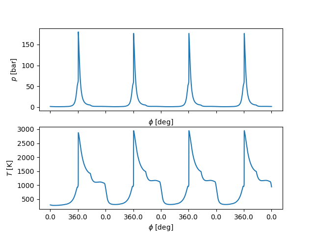
# pressure and temperature
xticks = np.arange(0, 0.18, 0.02)
fig, ax = plt.subplots(nrows=2)
ax[0].plot(t, states.P / 1.e5)
ax[0].set_ylabel('$p$ [bar]')
ax[0].set_xlabel(r'$\phi$ [deg]')
ax[0].set_xticklabels([])
ax[1].plot(t, states.T)
ax[1].set_ylabel('$T$ [K]')
ax[1].set_xlabel(r'$\phi$ [deg]')
ax[1].set_xticks(xticks)
ax[1].set_xticklabels(ca_ticks(xticks))
plt.show()

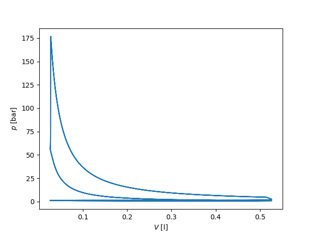
# p-V diagram
fig, ax = plt.subplots()
ax.plot(states.V[t > 0.04] * 1000, states.P[t > 0.04] / 1.e5)
ax.set_xlabel('$V$ [l]')
ax.set_ylabel('$p$ [bar]')
plt.show()

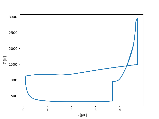
# T-S diagram
fig, ax = plt.subplots()
ax.plot(states.m[t > 0.04] * states.s[t > 0.04], states.T[t > 0.04])
ax.set_xlabel('$S$ [J/K]')
ax.set_ylabel('$T$ [K]')
plt.show()

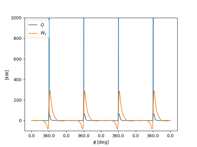
# heat of reaction and expansion work
fig, ax = plt.subplots()
ax.plot(t, 1.e-3 * states.heat_release_rate * states.V, label=r'$\dot{Q}$')
ax.plot(t, 1.e-3 * states.dWv_dt, label=r'$\dot{W}_v$')
ax.set_ylim(-1e2, 1e3)
ax.legend(loc=0)
ax.set_ylabel('[kW]')
ax.set_xlabel(r'$\phi$ [deg]')
ax.set_xticks(xticks)
ax.set_xticklabels(ca_ticks(xticks))
plt.show()

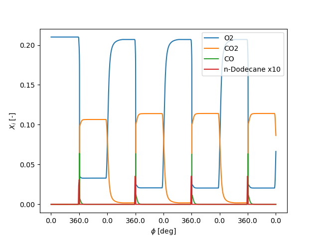
# gas composition
fig, ax = plt.subplots()
ax.plot(t, states('o2').X, label='O2')
ax.plot(t, states('co2').X, label='CO2')
ax.plot(t, states('co').X, label='CO')
ax.plot(t, states('c12h26').X * 10, label='n-Dodecane x10')
ax.legend(loc=0)
ax.set_ylabel('$X_i$ [-]')
ax.set_xlabel(r'$\phi$ [deg]')
ax.set_xticks(xticks)
ax.set_xticklabels(ca_ticks(xticks))
plt.show()

• 
• 
• 
• 
• 

Integral Results

# heat release
Q = trapz(states.heat_release_rate * states.V, t)
output_str = '{:45s}{:>4.1f} {}'
print(output_str.format('Heat release rate per cylinder (estimate):',
                        Q / t[-1] / 1000., 'kW'))

# expansion power
W = trapz(states.dWv_dt, t)
print(output_str.format('Expansion power per cylinder (estimate):',
                        W / t[-1] / 1000., 'kW'))

# efficiency
eta = W / Q
print(output_str.format('Efficiency (estimate):', eta * 100., '%'))

# CO emissions
MW = states.mean_molecular_weight
CO_emission = trapz(MW * states.mdot_out * states('CO').X[:, 0], t)
CO_emission /= trapz(MW * states.mdot_out, t)
print(output_str.format('CO emission (estimate):', CO_emission * 1.e6, 'ppm'))

Heat release rate per cylinder (estimate):   35.6 kW
Expansion power per cylinder (estimate):     18.5 kW
Efficiency (estimate):                       52.0 %
CO emission (estimate):                       8.9 ppm