This summer I've been working to add a dedicated steady-state solver to Cantera's ZeroD reactor network simulation module. Inspired by my study of ZeroD's current ODE time-integration solver, CVodesIntegrator (see this post), I developed a nonlinear algebraic solver class called Cantera_NonLinSol to be used by ReactorNet to solve the steady-state problem:

Class Cantera_NonLinSol: A nonlinear algebraic system solver, built upon Cantera's 1D multi-domain damped newton solver as a simplified interface.
- Implemented in Cantera_NonLinSol.h (see this on GitHub)

This blog post will go into detail about the mathematical theory behind solving steady-state reactor systems, and how Cantera_NonLinSol can be used to facilitate the process.

Steady-State Solution in `ReactorNet` Simulations¶

Steady-state is reached in a reactor when all internal state variables become constant while time advances, as different internal processes that would normally change these variables become perfectly balanced with each other. The governing equations discussed on Cantera’s Reactor Science page will still dictate the physical properties of the system, but their time derivatives become zero as properties become steady. This means that the governing equations, normally a system of ordinary differential equations, can be reduced to a system of nonlinear algebraic equations:

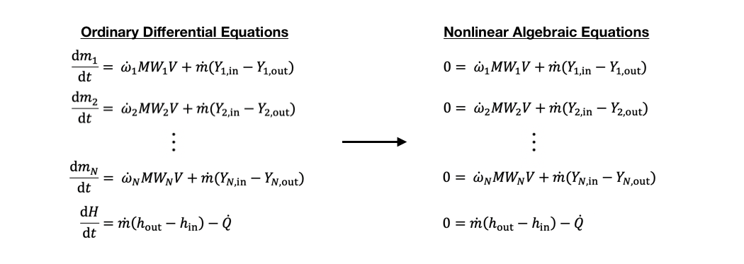
The system can now be solved with a nonlinear algebraic solver, which finds solution values for the state variables that will satisfy the system of equations. This means finding the zeroes to the functions defined on the right-hand-side of each equation. This is standard practice for any algebraic solution, and as such, nonlinear algebraic solvers typically require users to input a residual function that evaluates a specific system's right-hand-side functions.

Cantera has a built-in damped Newton/time-stepping hybrid solver, defined in the OneD module. This solver was designed for use with multiple-domain one-dimensional problems—this means that it can solve problems with several linked one-dimensional domains (each domain can have a different number of state variables), where solutions can be found at multiple spatial points within each physical domain. I designed Cantera_NonLinSol as a simplified interface to Cantera's solver, to solve a single system of nonlinear equations. This interface inputs problems to the Cantera 1D solver as single-domain, single-point systems. I used Cantera_NonLinSol within Cantera’s ZeroD module to solve the steady-state reactor equations and introduce basic steady-state solution capability.

What follows is a general outline of how to use this solver, with specific implementation examples included from my work in ZeroD:

Include the `Cantera_NonLinSol.h` header in your code.¶

ReactorNet.h, line 12 (see this on GitHub)

#include "cantera/numerics/Cantera_NonLinSol.h"

Derive a class from `Cantera_NonLinSol` to inherit nonlinear algebraic solution capabilities and define your specific problem.¶

ReactorNet.h, line 24 (see this on GitHub)

class ReactorNet : public FuncEval, public Cantera_NonLinSol

ReactorNet now exhibits multiple inheritance, since it was already a child of class FuncEval. The FuncEval parent class is used by Integrator during ODE time-integration, and its inheritance makes ReactorNet an ODE right-hand-side evaluator. (Confused? See my last blog post!)

Notice that the existing time-integration solver, Integrator, is not a parent class to ReactorNet. Integrator is an external solver object that uses user-defined functions from another class, FuncEval. This requires the inclusion of two headers, explicit construction of an external object, and the passing of the this pointer to locate user definitions:

ReactorNet.h, lines 10-11 (see this on GitHub)

#include "cantera/numerics/FuncEval.h"
#include "cantera/numerics/Integrator.h"

ReactorNet.cpp, line 18 (see this on GitHub)

m_integ(newIntegrator("CVODE")),

ReactorNet.cpp, line 112 (see this on GitHub)

m_integ->initialize(m_time, *this);

In contrast, Cantera_NonLinSol is written as an abstract base class that provides nonlinear algebraic solution capability to its children. User-defined function implementations are provided by overriding pure virtual functions declared in the parent class. Cantera_NonLinSol requires a single header inclusion, is automatically constructed by the child class, and can call user-provided functions without the use of a pointer.

Implement the problem-specific user-defined functions, to provide the solver with the number of equations (`ctNLS_nEqs()`), initial values (`ctNLS_initialValue()`), and residual function (`ctNLS_residFunction()`).¶

Steady-state solution is implemented using the same solution vector as in the transient case. This vector is a concatenation of solution vectors for each reactor in the network, with each sub-vector having the following format:

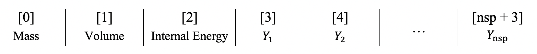
The size, m_nv, of the overall network solution vector is determined during ReactorNet initialization, and is returned by ctNLS_nEqs():

ReactorNet.cpp, lines 371-377 (see this on GitHub)

m_nv = 0;
m_start.assign(1, 0);
for (size_t n = 0; n < m_reactors.size(); n++) {
    Reactor& r = *m_reactors[n];
    m_nv += r.neq();
    m_start.push_back(m_nv);
}

ReactorNet.cpp, lines 397-400 (see this on GitHub)

size_t ReactorNet::ctNLS_nEqs()
{
    return m_nv;
}

Numerical solution of the steady-state equations is an initial-value problem, and as such it requires that ctNLS_initialValue() be implemented to provide a starting estimate for each component of the solution vector. In my ReactorNet implementation, the solution estimate is taken as the user-specified initial state of the network, and can be changed by modifying the contents of contained reactors. A good starting guess for a Reactor's steady-state solution is its inlet's state of fixed enthalpy/pressure chemical equilibrium, which can be obtained using ThermoPhase::equilibrate('HP').

In the source code, ReactorNet::ctNLS_initialValue() calls the initialValue() method of the appropriate Reactor, which returns the initial value of the requested solution component:

ReactorNet.cpp, lines 382-388 (see this on GitHub)

doublereal ReactorNet::ctNLS_initialValue(size_t i)
{
    for (size_t n = m_reactors.size() - 1; n >= 0; n--)
        if (i >= m_start[n])
            return m_reactors[n]->initialValue(i - m_start[n]);
    return -1;
}

Reactor.cpp, lines 547-559 (see this on GitHub)

doublereal Reactor::initialValue(size_t i) {
    m_thermo->restoreState(m_state);
    switch (i)
    {
    case 0:
        return m_thermo->density() * m_vol;
    case 1:
        return m_vol;
    case 2:
        return m_thermo->intEnergy_mass() * m_thermo->density() * m_vol;
    }
    return m_thermo->massFraction(i-3);
}

Lastly, the residual function that defines the specific nonlinear algebraic system needs to be specified in ctNLS_residFunction(). In the case of a reactor network, calculation of the residual requires chemical kinetics properties based on the current solution approximation. For this, the state of each reactor is updated based on several steady-state assumptions:

The mass flow rate is constant, and the inflow rate equals the outflow rate.
Reactor volume is constant.
Reactor pressure is constant.
The total specific enthalpy at the inlets equals the total specific enthalpy at the outlets (and within the reactor).

These assumptions allow updating a Reactor's internal state based on the known pressure and specific enthalpy, along with the iteration mass fractions computed by the solver. Residuals for mass, volume, and energy are set based on corresponding values in the updated reactor, while species conservation residuals are calculated using the built-in evalEqs() method:

Reactor.cpp, lines 500-543 (see this on GitHub)

void Reactor::residFunction(double *sol, double *rsd)
{
    doublereal Hdot = 0;
    doublereal mdot = 0;
    evalFlowDevices(0);
    for (size_t i = 0; i < m_inlet.size(); i++) {
        Hdot += m_mdot_in[i] * m_inlet[i]->enthalpy_mass();
        mdot += m_mdot_in[i];
    }
    doublereal h = Hdot/mdot;
    m_thermo->restoreState(m_state);
    doublereal p = m_thermo->pressure();
    m_thermo->setMassFractions_NoNorm(sol+3);
    m_thermo->setState_HP(h,p);
    syncState();
    evalEqs(0, sol, rsd, 0);
    rsd[0] = m_mass - sol[0];
    rsd[1] = m_vol - sol[1];
    rsd[2] = m_intEnergy*m_mass - sol[2];
}

Call the inherited `solve()` function, which will update the network to its steady-state.¶

ReactorNet.cpp, line 379 (see this on GitHub)

Cantera_NonLinSol::solve();

Note that the Cantera_NonLinSol namespace is included in this call only for clarity.

This solver is still in its initial development phase, and feedback or suggestions you may be able to provide would definitely contribute to its success! Leave me a comment on GitHub, the Cantera User's Group, or email me at paul_d_blum@yahoo.com.

Thanks for reading!

@paulblum

Keep Reading:¶

Next Post - GSoC 2020 Project Summary

Previous Post - GSoC 2020 Blog Post 3

Start from the Beginning - Introduction

Steady-State Solution in ReactorNet Simulations¶

Include the Cantera_NonLinSol.h header in your code.¶

Derive a class from Cantera_NonLinSol to inherit nonlinear algebraic solution capabilities and define your specific problem.¶

Implement the problem-specific user-defined functions, to provide the solver with the number of equations (ctNLS_nEqs()), initial values (ctNLS_initialValue()), and residual function (ctNLS_residFunction()).¶

Call the inherited solve() function, which will update the network to its steady-state.¶